0. Introduction
This set of files contains monthly and decadal summaries of marine data for the years 1854 through 1979, separated into 2° latitude x 2° longitude boxes. Details of the packed binary formats, field explanations, and the method used for computing the different variables and statistics that make up the summaries are all documented. Much of the documentation is referred to by and is essential to understand supp. B and supp. C. The reduced-volume group files (supp. B) offer a manageable alternative, in terms of processing and storage costs, for studies using only a few variables and statistics. The derivation and format of the limits used as a basis for eliminating outliers from a portion of the summaries, together with other information about this statistical trimming process, are covered in supp. C.
1. Variables and Statistics
The 19 weather variables shown in Table A1-1 were summarized; for notational purposes each is assigned an UPPERCASE ITALIC letter called β.
----------------------------------------------------------------------
 #   β    Variable
----------------------------------------------------------------------
                              "Observed"
 1   S    sea surface temperature
 2   A    air temperature
 3   W    scalar wind
 4   U    vector wind eastward component
 5   V    vector wind northward component
 6   P    sea level pressure
 7   C    total cloudiness
 8   Q    specific humidity

----------------------------------------------------------------------
                               Derived
 9   R    relative humidity
10   D    S - A = sea-air temperature difference
11   E    (S - A)W = sea-air temperature difference*wind magnitude
12   F    Qs - Q = (saturation Q at S) - Q
13   G    FW = (Qs - Q)W (evaporation parameter)
14   X    WU
15   Y    WV (14-15 are wind stress parameters)
16   I    UA
17   J    VA
18   K    UQ
19   L    VQ (16-19 are sensible and latent heat transport parameters)
----------------------------------------------------------------------
For each of these variables the 14 statistics shown in Table A1-2 are included; each is assigned a lowercase italic character called α.
---------------------------------------------------
 #   α    Statistic
---------------------------------------------------
 1   d    mean day-of-month of observations
 2   h    hour statistic of observations
 3   x    mean longitude of observations
 4   y    mean latitude of observations
 5   n    number of observations
 6   m    mean
 7   s    standard deviation
 8   0    0/6 sextile (the minimum)
 9   1    1/6 sextile (a robust estimate of m - 1s)
10   2    2/6 sextile
11   3    3/6 sextile (the median)
12   4    4/6 sextile
13   5    5/6 sextile (a robust estimate of m + 1s)
14   6    6/6 sextile (the maximum)
---------------------------------------------------
NOTE: these summaries were prepared for two conditions:
2. Monthly Summaries
Each logical record within the Monthly Summaries Trimmed (MST) or the Monthly Summaries Untrimmed (MSU) contains all the data for an individual year-month-2° box, organized primarily by statistic, within which by variable. For example, letting αβ denote the value of the statistic α for the variable β, each summary in the untrimmed file contains
((αβ, β = S,...,Q), α = d,...,6)
which defines the following matrix, with 8 rows and 14 columns:
   | α |  d   h   x   y   n   m   s   0   1   2   3   4   5   6
---|---|--------------------------------------------------------
 β | # |  1   2   3   4   5   6   7   8   9  10  11  12  13  14
---|---|--------------------------------------------------------
 S | 1 | dS  hS  xS  yS  nS  mS  sS  0S  1S  2S  3S  4S  5S  6S
 A | 2 | dA  hA  xA  yA  nA  mA  sA  0A  1A  2A  3A  4A  5A  6A
 W | 3 | dW  hW  xW  yW  nW  mW  sW  0W  1W  2W  3W  4W  5W  6W
 U | 4 | dU  hU  xU  yU  nU  mU  sU  0U  1U  2U  3U  4U  5U  6U
 V | 5 | dV  hV  xV  yV  nV  mV  sV  0V  1V  2V  3V  4V  5V  6V
 P | 6 | dP  hP  xP  yP  nP  mP  sP  0P  1P  2P  3P  4P  5P  6P
 C | 7 | dC  hC  xC  yC  nC  mC  sC  0C  1C  2C  3C  4C  5C  6C
 Q | 8 | dQ  hQ  xQ  yQ  nQ  mQ  sQ  0Q  1Q  2Q  3Q  4Q  5Q  6Q
stored in the order:
Because of the matrix organization it is possible to address each αβ by its row and column number, e.g., sW = MSU(3,7). The FORTRAN programmer may find it convenient to store this matrix in an array such as DIMENSION MSU (8,14). For this reason, the tables that describe the bit layout of each format are presented in two parts: the first gives the column organization and the second gives the row organization, with column or row indices along the left-hand margin.
An MSU was output if and only if at least one report (supp. E) fell within a year-month-2° box, regardless of whether it is landlocked (according to supp. G). This happened even if there were no acceptable observations of any variable, in which case the MSU had the code zero output for missing data in each αβ. In contrast, an MST was output only if at least one acceptable (not trimmed) observation was found in a non-landlocked 2° box.
2.1 Monthly Summaries Trimmed (MST)
These were derived from the trimmed data that had outliers
removed by a statistical process. Table A2-1a shows the bit layout of
each MST and Table A2-1b shows the bit layout of each of its 152-bit
or 304-bit sections, in sequential bit-order reading from top to
bottom.
 #   α     Statistic                                 Bits
---------------------------------------------------------
           rptin                                       16
           year                                         8
           month                                        4
           2° box                                      14
           10° box                                     10
           checksum                                    12
---------------------------------------------------------
 1   d     mean day-of-month of observations          152
 2   ht    fraction of observations in daylight       152
 3   x     mean longitude of observations             152
 4   y     mean latitude of observations              152
 5   n     number of observations                     304
 6   m     mean                                       304
 7   s     standard deviation                         304
 8   0     0/6 sextile (the minimum)                  304
 9   1     1/6 sextile (a robust estimate of m - 1s)  304
10   2     2/6 sextile                                304
11   3     3/6 sextile (the median)                   304
12   4     4/6 sextile                                304
13   5     5/6 sextile (a robust estimate of m + 1s)  304
14   6     6/6 sextile (the maximum)                  304
---------------------------------------------------------
           total                                     3712
 #   β    Variable                         Bits   Bits
------------------------------------------------------
 1   S    sea surface temperature             8     16
 2   A    air temperature                     8     16
 3   W    scalar wind                         8     16
 4   U    vector wind eastward component      8     16
 5   V    vector wind northward component     8     16
 6   P    sea level pressure                  8     16
 7   C    total cloudiness                    8     16
 8   Q    specific humidity                   8     16
 9   R    relative humidity                   8     16
10   D    S - A                               8     16
11   E    (S - A)W                            8     16
12   F    Qs - Q = (saturation Q at S) - Q    8     16
13   G    FW                                  8     16
14   X    WU                                  8     16
15   Y    WV                                  8     16
16   I    UA                                  8     16
17   J    VA                                  8     16
18   K    UQ                                  8     16
19   L    VQ                                  8     16
------------------------------------------------------
          total                             152    304
These were derived from the untrimmed data that had only gross
errors removed. Table A2-2a shows the bit layout of each MSU and Table
A2-2b shows the bit layout of its 64-bit or 128-bit sections, in
sequential bit-order reading from top to bottom.
 #   α     Statistic                                    Bits
------------------------------------------------------------
           rptin                                          16
           year                                            8
           month                                           4
           2° box                                         14
           10° box                                        10
           checksum                                       12
------------------------------------------------------------
 1   d     mean day-of-month of observations*             64
 2   hu    mean hour of observations                      64
 3   x     mean longitude of observations                 64
 4   y     mean latitude of observations                  64
 5   n     number of observations                        128
 6   m     mean                                          128
 7   s     standard deviation                            128
 8   0     0/6 sextile (the minimum)                     128
 9   1     1/6 sextile (a robust estimate of m - 1s)     128
10   2     2/6 sextile                                   128
11   3     3/6 sextile (the median)                      128
12   4     4/6 sextile                                   128
13   5     5/6 sextile (a robust estimate of m + 1s)     128
14   6     6/6 sextile (the maximum)                     128
------------------------------------------------------------
           total                                        1600

* In conversion from MSU.1 to MSU.2, units of mean day were
reduced in precision from 0.1 to 0.2, by rounding all odd
tenths positions up.  Because of previous rounding, the new
mean days will tend to overestimate; e.g., a mean day of 1.4
actually signifies a mean day in the interval [1.25,1.45),
centered under 1.35. To obtain the midpoint use a base of
3.75 instead of 4 as shown in Table A2-4a, except that 1.025
and 30.925 are the two extreme midpoints.
__________________________
 #   β    Variable                        Bits   Bits
-----------------------------------------------------
 1   S    sea surface temperature            8     16
 2   A    air temperature                    8     16
 3   W    scalar wind                        8     16
 4   U    vector wind eastward component     8     16
 5   V    vector wind northward component    8     16
 6   P    sea level pressure                 8     16
 7   C    total cloudiness                   8     16
 8   Q    specific humidity                  8     16
-----------------------------------------------------
           total                            64    128
It is assumed that the reader is familiar with techniques for transferring a binary block into memory and then extracting into INTEGER variables the bit strings whose lengths are given in Tables A2-1a and A2-1b or A2-2a and A2-2b. Refer to supp. H for more information. For a general discussion including the advantage in execution time and storage relative to traditional techniques see [3].
Compression was achieved by packing data represented as positive integers into fields whose lengths are specified in the bits column of Tables A2-1a and A2-1b or A2-2a and A2-2b. To accomplish this, a field's floating point true value was divided by its units (the smallest increment of the data that has been encoded). After rounding, a base was subtracted to produce the coded positive integer, which was finally right-justified with zero fill in the field's position within the summary. Using the mS true value 28.61°C as an example, (28.61/0.01) - (-501) = 3362.
Once a given field has been extracted into the coded value, the true value can be reconstructed by reversing the process:
true value = (coded + base) * unitsThe above true value example is reconstructed by (3362 + (-501)) * 0.01) = 28.61°C.
The coded and true value ranges, the units, and the base associated with each α statistic will be found in Table A2-4a; the hour statistic is different for MST and MSU, hence the subscript on the two different entries. In the case of means, standard deviations, and sextiles these quantities are different for each β variable, hence cross-reference to Table A2-4b. For the identification fields that prefix each summary these quantities will be found in Table A2-4c.
As a representative example, suppose that the untrimmed coded
values shown in Table A2-3a have been unpacked into FORTRAN INTEGER
variables whose name is αβ prefixed by I.
Name    Coded value
-------------------
IdS             151
IhA              98
IxW              56
IyU               0
InV              43
ImP           14140
IsC              25
I0Q             372
-------------------
Instruction               Name         True value
-------------------------------------------------
dS = (IdS + 4) * 0.2        dS          31.0 days
hA = (IhA - 1) * 0.1        hA          9.7 hours
xW = (IxW - 1) * 0.01       xW              0.55°
if(IyU.EQ.0)then            yU            missing
nV = (InV + 0) * 1          nV                43.
mP = (ImP + 86999) * 0.01   mP         1011.39 mb
sC = (IsC - 1) * 0.1        sC           2.4 okta
0Q = (I0Q - 1) * 0.01       0Q        3.71 g kg-1
-------------------------------------------------
#    α   Statistic                   True value      Units*        Base        Coded
----------------------------------------------------------------------------------------
1    d   mean day-of-month of obs    1.0≤31.0**      0.2 day         4         1≤151
2    ht  fraction of obs in daylight 0.00≤1.00       0.01           -1         1≤101
2    hu  mean hour of obs            0.0≤23.0        0.1 hour       -1         1≤231
3    x   mean longitude of obs       0.00≤2.00       0.01°          -1         1≤201
4    y   mean latitude of obs        0.00≤2.00       0.01°          -1         1≤201
5    n   number of obs               1≤65535         1               0         same
6    m   mean                        Table A2-4b   Table A2-4b  Table A2-4b  Table A2-4b
7    s   standard deviation          0≤***         Table A2-4b      -1         1≤***
8-14 0-6 sextiles                    Table A2-4b   Table A2-4b  Table A2-4b  Table A2-4b
----------------------------------------------------------------------------------------

* "Units" gives the smallest increment of the data that has been encoded. Thus a change
of one unit in the integer coded value represents a change in the true value of one of
the units shown.
** m ≤ n denotes "from m through n inclusive."
*** Standard deviations have a true value ranging upwards from zero for all variables,
thus the base is always -1. Units for each variable are still chosen from Table A2-4b.
__________________________
 #  β  Variable               True value     Units             Base   Coded
-----------------------------------------------------------------------------
        "Observed"
 1  S  sea surface
       temperature           -5.00≤40.00    0.01 °C            -501   1≤4501
 2  A  air temperature      -88.00≤58.00    0.01 °C           -8801   1≤14601
 3  W  scalar wind            0.00≤102.20   0.01 m s-1           -1   1≤10221
 4  U  vector wind
       eastward component  -102.20≤102.20   0.01 m s-1       -10221   1≤20441
 5  V  vector wind
       northward component -102.20≤102.20   0.01 m s-1       -10221   1≤20441
 6  P  sea level pressure   870.00≤1074.60  0.01 mb           86999   1≤20461
 7  C  total cloudiness        0.0≤8.0      0.1 okta             -1   1≤81
 8  Q  specific humidity      0.00≤40.00    0.01 g kg-1          -1   1≤4001
-----------------------------------------------------------------------------
         Derived
 9  R  relative humidity       0.0≤100.0    0.1%                 -1   1≤1001
10  D  S - A                -63.00≤128.00   0.01 °C           -6301   1≤19101
11  E  (S - A) W           -1000.0≤1000.0   0.1 °C m s-1     -10001   1≤20001
12  F  Qs - Q = (saturation
       Q at S) - Q          -40.00≤40.00    0.01 g kg-1       -4001   1≤8001
13  G  FW                  -1000.0≤1000.0   0.1 g kg-1 m s-1 -10001   1≤20001
14  X  WU                  -3000.0≤3000.0   0.1 m2 s-2       -30001   1≤60001
15  Y  WV                  -3000.0≤3000.0   0.1 m2 s-2       -30001   1≤60001
16  I  UA                  -2000.0≤2000.0   0.1 °C m s-1     -20001   1≤40001
17  J  VA                  -2000.0≤2000.0   0.1 °C m s-1     -20001   1≤40001
18  K  UQ                  -1000.0≤1000.0   0.1 g kg-1 m s-1 -10001   1≤20001
19  L  VQ                  -1000.0≤1000.0   0.1 g kg-1 m s-1 -10001   1≤20001
-----------------------------------------------------------------------------
 Field    True value  Units    Base     Coded
----------------------------------------------
 RPTIN       n/a       n/a      n/a      n/a
  year    1800≤2054     1      1799     1≤255
 month      1≤12        1         0      same
 2° box    1≤16202      1         0      same
10° box     1≤648       1         0      same
checksum     n/a       n/a      n/a      n/a
----------------------------------------------
These bits are reserved for use of the RPTIN unblocking utility, where available (e.g., NCAR). Otherwise they may be ignored.
The year can range from 1800 to 2054.
1=January,2=February,...,12=December.
See supp. G for a description of the 2° and 10° box systems, and supp. H for related software.
A checksum was computed and stored with each packed summary as a measure of reliability during storage and transmission. For both untrimmed and trimmed summaries, the checksum is computed by
Repeating this calculation for every unpacked summary, and then verifying that the checksum so obtained agrees with the coded checksum stored in the summary, is strongly encouraged. For example, supposing that the coded untrimmed data matrix is available in an array MSU, the checksum CK is computed and verified against the stored checksum CKS in FORTRAN as follows:
          INTEGER CK,J,I,MSU(8,14),YEAR,MONTH,BOX2,BOX10,CKS
          CK = 0
          DO 500 J = 1,14
              DO 400 I = 1,8
                  CK = CK + MSU(I,J)
     400      CONTINUE
     500  CONTINUE
          CK = CK + YEAR + MONTH + BOX2 + BOX10
          CK = MOD(CK,4095)
          IF(CK .NE. CKS) THEN
              PRINT *,'ERROR. CK = ',CK,' .NE. CKS = ',CKS
              STOP
          ENDIF
Note that using modulus 212-1 takes into account every bit of CK, versus chopping at the twelfth bit using modulus 212.
3. Decadal Summaries
Each logical record within the Decadal Summaries Trimmed (DST) or the Decadal Summaries Untrimmed (DSU) contains all the data for an individual decade-month-2° box, organized primarily by variable, within which by statistic. (NOTE: this organization is transposed from that of the monthly summaries.)
A DSU was output if and only if at least one report (supp. E) fell within a decade-month-2° box, regardless of whether it is landlocked (according to supp. G). This happened even if there were no acceptable observations of any variable, in which case the DSU had the code zero output for missing data in each αβ. In contrast, a DST was output only if at least one acceptable (not trimmed) observation was found in a non-landlocked 2° box.
3.1 Decadal Summaries Trimmed (DST)
Table A3-1a shows the bit layout of each DST and Table A3-1b
shows the bit layout of each of its 160-bit sections, in sequential
bit-order reading from top to bottom.
 #   β    Variable                         Bits
-----------------------------------------------
          rptin                              16
          decade                              8
          month                               4
          2° box                             14
          10° box                            10
          checksum                           12
-----------------------------------------------
 1   S    sea surface temperature           160
 2   A    air temperature                   160
 4   U    vector wind eastward component    160
 5   V    vector wind northward component   160
 6   P    sea level pressure                160
 8   Q    specific humidity                 160
 9   R    relative humidity                 160
-----------------------------------------------
          (ΣUV)/n                            32
          (ΣU2)/n                            32
          (ΣV2)/n                            32
-----------------------------------------------
          total                            1280
 #   α    Statistic                                 Bits
--------------------------------------------------------
 5   n    number of observations                      16
 6   m    mean                                        16
 7   s    standard deviation                          16
 8   0    0/6 sextile (the minimum)                   16
 9   1    1/6 sextile (a robust estimate of m - 1s)   16
10   2    2/6 sextile                                 16
11   3    3/6 sextile (the median)                    16
12   4    4/6 sextile                                 16
13   5    5/6 sextile (a robust estimate of m + 1s)   16
14   6    6/6 sextile (the maximum)                   16
--------------------------------------------------------
          total                                      160
Table A3-2a shows the bit layout of each DSU and Table A3-2b
shows the bit layout of each of its 128-bit sections, in sequential
bit-order reading from top to bottom.
 #   β    Variable                         Bits
-----------------------------------------------
          rptin                              16
          decade                              8
          month                               4
          2° box                             14
          10° box                            10
          checksum                           12
-----------------------------------------------
 1   S    sea surface temperature           128
 2   A    air temperature                   128
 4   U    vector wind eastward component    128
 5   V    vector wind northward component   128
 6   P    sea level pressure                128
 9   R    relative humidity                 128
-----------------------------------------------
          mean of U                          16
          mean of V                          16
          (ΣUV)/n                            32
          (ΣU2)/n                            32
          (ΣV2)/n                            32
-----------------------------------------------
          total                             960
 #   α    Statistic                                 Bits
--------------------------------------------------------
 8   0    0/6 sextile (the minimum)                   16
 9   1    1/6 sextile (a robust estimate of m - 1s)   16
10   2    2/6 sextile                                 16
11   3    3/6 sextile (the median)                    16
12   4    4/6 sextile                                 16
13   5    5/6 sextile (a robust estimate of m + 1s)   16
14   6    6/6 sextile (the maximum)                   16
 5   n    number of observations                      16
--------------------------------------------------------
          total                                      128
The coded and true value ranges, the units, and the
base for the decadal fields that are unique to the decadal summaries
are given in Table A3-3. All other decadal fields are common to the monthly summaries,
with characteristics as given in sec. 2.3.
Field      True value        Units       Base        Coded
--------------------------------------------------------------
decade     180≤205           1           179         1≤26
(ΣUV)/n    -5222.42≤5222.42  0.01 m s-1  -522243     1≤1044485
(ΣU2)/n    0≤10444.84        0.01 m s-1  -1          1≤1044485
(ΣV2)/n    0≤10444.84        0.01 m s-1  -1          1≤1044485
--------------------------------------------------------------
This is simply the true value YEAR with the units position
omitted; i.e., using INTEGER truncating arithmetic,
DECADE=YEAR/10
A variance /covariance matrix can be obtained using these plus the mean of U and V, where n is from either U or V.
4. Computational Method
The method of computing all the different statistics and variables is given, together with the computational dependencies of the variables on each other. The data used as a basis for trimming and their derivation are described in supp. C.
4.1 Statistics
The method of computing statistics is the same for all variables. (The method of computing the fraction of observations observed in daylight is described in sec. 4.2; here h refers to hu .) Let ai denote either a single observation of one variable, or, where applicable, a single measure of observational location: the day, hour, latitude, or longitude it was taken at.
Let M represent any one of the five mean statistics d, h, x, y, m computed for the n ai by
for n> 0. For each of x, y, and m, n = n (n is the number of observations in the summary); for d and h, n ≤ n because an individual day or hour may be missing. Consequently, the means d or h may be missing when x, y, and m are not.
The standard deviation s about the mean m is then
for n > 1, or s = 0 if n = 1.
To compute the sextiles 0, 1, 2, 3, 4, 5, 6, the observations must first be ranked in ascending order such that ai ≤ ai + 1 for any i < n. Ordinarily, each sextile, sj, would be
But the (j/6) for j = 1 and 5 have been adjusted slightly to 0.1587 and 0.8413, in order to correspond to the cumulative area under the standardized normal (m = 0; s = 1) curve at ≤ - 1 and ≤ + 1 standard deviations, respectively. Also, (j modulo 6) is guaranteed to be zero only at j = 0 and 6. In all but the case of the minimum and maximum, instead of (3), first
         (j/6)(n-1)+1        for j = 2,3,4,
f   =    (0.1587)(n-1)+1     for j = 1,       (Eq. 4)
         (0.8413)(n-1)+1     for j = 5,
using floating point arithmetic. Second, letting k equal the integer part of f
Equation (5) does a linear interpolation to the jth sextile, sj, (f-k) of the distance between ak and ak + 1, in case f has a fractional part.
The sextiles were actually computed (using FORTRAN) from an INTEGER histogram whose stepsize and length represent one-tenth the units and true value range, respectively, required for a particular variable by Table A2-4b (i.e., reduced in each case by omitting the least significant decimal place). Variables that were computed to floating point precision, rather than available directly as fields in the input report (see sec. 4.3), were rounded to the nearest histogram step. Since the mean m and standard deviation s were computed separately using floating point data before rounding, the median and mean may differ slightly in cases where they would be identical using infinite-precision arithmetic.
4.2 Fraction of Observations in Daylight
When the east longitude X and HOUR in GMT of a report are used, the absolute hour difference of the report from local solar noon is
with a modulus of 24 in case the report falls in the local solar day succeeding the GMT day (the possible effect of this day crossover on local solar month is ignored). For the two polar 2° boxes, X is zero by convention.
A report is said to fall in daylight if t is no greater than Δt, the half length of the duration of daylight, in which case a separate counter k for each variable is incremented (only provided the observation of that variable is extant and not trimmed):
Upon completion of a year-month-2° box containing n observations of one variable, the statistic ht (the fraction of reports in daylight) is
For computational efficiency, a 12 months x 90 latitudes table of
representative values for Δt was derived from the declination
angle of the sun δ at the middle of each month, as listed in
Table A4-1, and from the middle latitude y1 of each zone of
2° boxes (89°N, 87°N,...,89°S).
  Mid-month         δ
------------------------
16 January       -21.16
15 February      -13.09
16 March          -2.22
15.5 April         9.51
16 May            18.81
15.5 June         23.285
16 July           21.57
16 August         14.14
15.5 September     3.315
16 October        -8.43
15.5 November    -18.31
16 December      -23.27
------------------------
except that in case the absolute value of the right-hand side of (9) exceeds one (within the Arctic or Antarctic Circles), the right-hand side retains its sign but assumes an absolute value of one. Finally, τ0 degrees converts to Δt hours by
since 360 degrees corresponds to 24 hours.
4.3 Variables
The first seven "observed" variables are available directly as
fields in the input report (S, A, W, U,
V, P, C) although [U V]' is
actually observed as magnitude W and direction D; Q and the eleven
other variables are derived from these or one other report field: dew
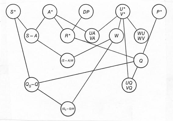
point depression DP. A variable is not computed if it is dependent on
a variable that is missing or has been trimmed. Table A4-2 lists the
report fields (from supp. E) that are necessary to compute each
variable; Figure A4-1 illustrates the order in which variables are
computed and trimmed, including other dependencies.
                              Report field
 Variable         S    A    DP   W    U    V    P    C
-------------------------------------------------------
"Observed"
S                 X
A                      X
W                                X
U                                     X
V                                          X
P                                               X
C                                                    X
Q                      X    X                   X
-------------------------------------------------------
 Derived
R                      X    X
S - A             X    X
(S - A)W          X    X         X
Qs - Q            X    X    X                   X
(Qs - Q)W         X    X    X    X              X
WU                               X    X
WV                               X         X
UA                     X              X
VA                     X                   X
UQ                     X    X         X         X
VQ                     X    X              X    X
-------------------------------------------------------
Figure A4-1. Variable hierarchy. In order for a variable to be computed, the variables that are connected to it and above it must have been computed to fall within their respective true value ranges and not be trimmed. All the nodes are applicable only to MST; an asterisk marks the explicitly trimmed variables. For other products the appropriate sub-graph still applies, with two untrimmed exceptions: 1) although R does not appear in MSU, one condition for Q is that R be successfully computed for DSU; and 2) in MSU and DSU, an observation of W is accepted even if U and V are missing (because of a report containing wind speed without direction). The paired variables, which are all functions of U and V, appear in the same node -- but processing of the U function actually precedes processing of the V function. Also, processing is never reversed; e.g., if R is trimmed A is not reprocessed.
4.4 Moisture Variables
The derived moisture variables (Q, R, and Qs) are computed using the FORTRAN functions that are given in [10] and referenced as follows:
     Q  = SSH(P,A - DP)
     R  = HUM(A,A - DP)
     Qs = SSH(P,S)
Inside SSH the mixing ratio is approximated by function WMR. The
method of computing vapor pressure differs in the untrimmed and
trimmed summaries. Function ESLO was used in the untrimmed summaries.
Unfortunately, ESLO is unreliable at physically unrealistic
conditions, although tests have demonstrated that, at least, no R
exceeded 100%. Function ES was used instead in the trimmed summaries.
These algorithms were chosen because of their accuracy and
computational efficiency. For more detailed information including the
original source of these techniques see [10].