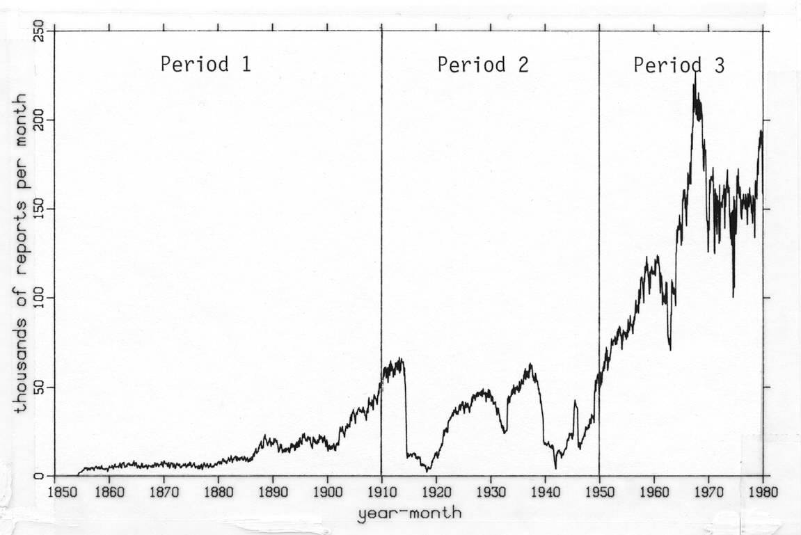
Figure C1-1. Global reports after duplicate elimination, divided into periods that separate limits were established for using untrimmed data.
0. Introduction
Secs. 1 and 2 define trimming and describe smoothing methods used to derive the Decadal Summary Untrimmed Limits (DSUL). These limits were input to the second statistics pass as a basis for rejecting (trimming) data. Secs. 3 and 4 detail the format for DSUL and for the data that measure Trimming Performance (TRP).
Cross reference is made to supp. A for standardized unpacking information, and the same notation for variables and statistics is followed or extended, also using the same type of two-dimensional table presentation.
1. Trimming
In the first statistics pass, the untrimmed monthly and decadal summaries (MSU and DSU) were generated. The untrimmed decadal summaries were used to derive a set of upper and lower limits (DSUL) for the variables S, A, U, V, P, R. In the second statistics pass, each individual observation of one of these variables was "trimmed" if it fell outside the limits in DSUL. This had the effect of rejecting such an observation from the trimmed monthly and decadal summaries (MST and DST). Since other variables W, Q, D, E, F, G, X, Y, I, J, K, L are all functions of two or more of the explicitly trimmed variables, they were computed only if the variables they depend on survived computation and trimming (see Figure A4-1 in supp. A). Total cloudiness C was not trimmed, and its "trimmed" and untrimmed statistics would be identical, except for differences in input data (see supp. A).
Bivariate techniques that were considered for trimming the wind vector [U V]', such as one based on squared statistical distance [4], were abandoned because of their sensitivity to outliers and the infeasibility of multiple passes through the data. Instead, each component was treated exactly like a univariate quantity in trimming, and both (plus the wind magnitude W) were trimmed if either U or V failed.
There are two additional products from trimming. First, individual observations of the explicitly trimmed variables were flagged by their Compressed Marine Reports (see supp. D) to show if they were trimmed as outliers or for other reasons. When an individual observation was trimmed, it was omitted from the trimmed summaries, but was not omitted from CMR. Instead a flag was set in the CMR file, thus making that file a source of both untrimmed and trimmed data. Second, trimming performance was measured by data described in sec. 4.
An individual observation ai of any variable i (i = S,A,U,V,P,R) was trimmed if it fell outside its lower or upper limit:
where p is the final year of the period (1909, 1949, 1979), m is the month (1,...,12), and b is the 2° box (1,...,16202) that contain ai. The three periods,
1854-1909 (6 decades)were chosen to keep the trimming criteria separate, in general, across possible climatic epochs or instrumental and observational discontinuities (see Figure C1-1).
1910-1949 (4 decades)
1950-1979 (3 decades)
Figure C1-1. Global reports after duplicate elimination, divided into periods that separate limits were established for using untrimmed data.
Further, an individual observation was automatically trimmed if the 2° box was landlocked according to the approximate table given in supp. G, or if the lower and upper limits were missing. Both the values "missing" and "landlocked" are defined in DSUL.
2. Derivation of Smoothed Limits
The lower and upper limits lipmb and uipmb (in subsequent material referred to simply as l and u) depend on
i = variable (S, A, U, V, P, R)They were derived from the 1/6, 3/6 (median), and 5/6 decadal sextiles (s1, s3, s5) in the untrimmed decadal summaries, using smoothing operations across time-related or space-adjacent 2° boxes, within a period, and then applying additional smoothing and other steps to create the final limits contained in DSUL. This extensive smoothing was done to reduce as much as possible the effect of outliers on l and u, since distorted limits might trim out perfectly good observations.
p = period (1854-1909, 1910-1949, 1950-1979)
m = month (January,...,December)
b = box (1,...,16202)
The decadal sextiles (s1, s3, s5) were used as input to the smoothing process because they were considered less sensitive to outliers in the original untrimmed data than a decadal mean m or standard deviation s. The median s3 is an estimator of m, and the quantities (s3 - s1) and (s5 - s3), called mdevl and mdevu (for median-deviation-lower and -upper), are estimators of -1s and +1s, respectively. Assuming a normal distribution, the relationship
tends to equality as random sample-size increases, where e = (s5 - s1)/2 is available in group files (supp. B). Otherwise, asymmetry in a distribution may be recognized using (s3 - s1) and (s5 - s3) separately.
First, each of the DSU data were tested for reasonableness. For the decadal medians, the data were rejected (i.e., set to "landlocked") if the box was located on land. The deviations (s3 - s1) and (s5 - s3) were rejected if on land or if the number of observations n from which they were derived was less than 3 (the medians s3 were included for all n > 0).
2.1 Decadal Cubes
A given 2° box, b, together with those boxes adjacent in longitude x and latitude y makes a group of nine, as shown by Figure C2-1.
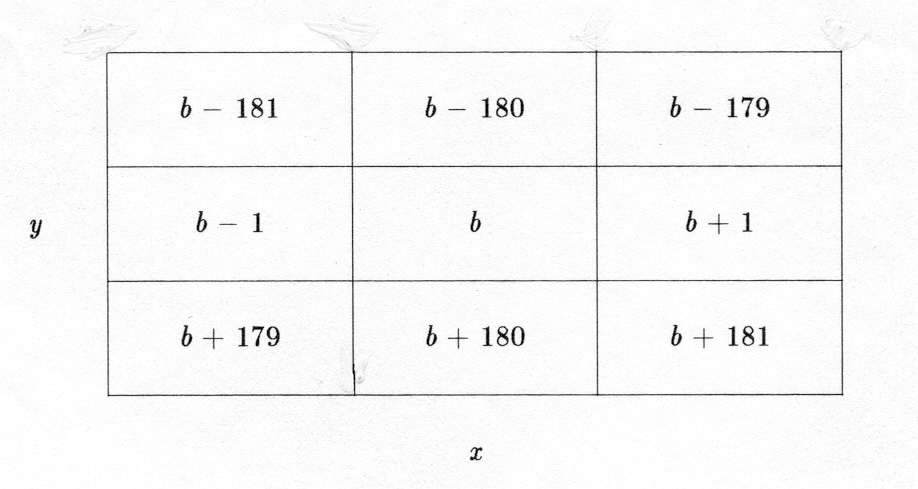
Figure C2-1. 2° boxes geographically-contiguous to b. Procedures were modified when b has as its boundary 0° longitude, so as to include the geographically contiguous boxes, or when b is one of the polar or polar-adjacent boxes.
Adding a similar group from the preceding month in the same decade and also one from the following month yields a cube in latitude, longitude, and month, similar to "Rubik's Cube" (Figure C2-2). The decadal cube has 27 possible sets of s3, (s3 - s1), and (s5 - s3), one central set and the others in pairs symmetric about the center.
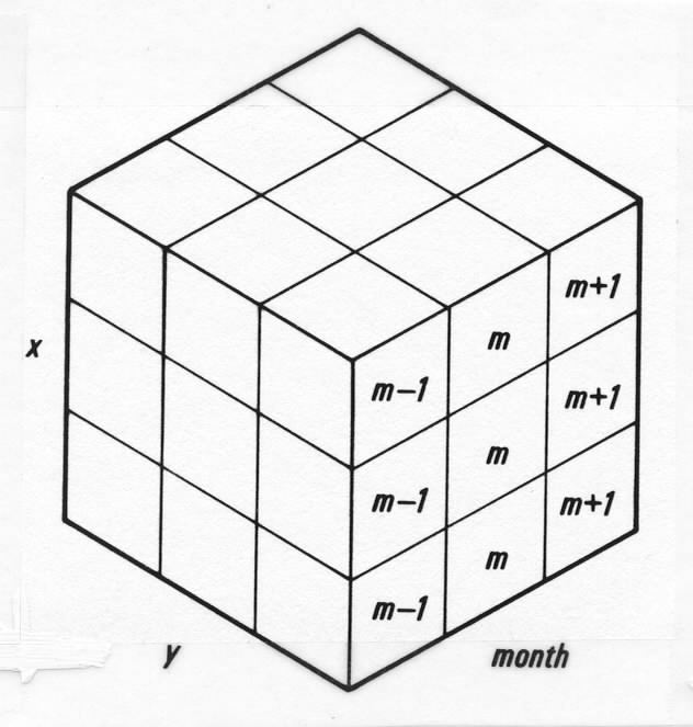
Figure C2-2. Decadal cube example.
For each of the three periods, cubes were constructed around a given central box for each decade in the period (except for the number of decades, the procedure was the same for each variable-period-2° box-month). Let M represent the number of medians (s3), and N represent the number of deviations (s3 - s1) and (s5 - s3), found jointly in all the decadal cubes centered on a box in one period. Thus 162, 108, or 81 is the maximum for M and N, depending on whether the period contains 6, 4, or 3 decades.
Of course M or N may be reduced below the maximum because of missing or landlocked data, and the requirement that deviations have n > 2 allows the possibility that N ≤ M. In addition, to preserve spatial or temporal gradients centered in a decadal cube, the symmetric pairs were included only when both members of a pair were present. If one of the pair was missing or landlocked, the other was set to missing.
Three statistics were generated using the surviving M values of s3, and N sets of (s3 - s1) and (s5 - s3):
σ1 = median of the N values of (s3 - s1) (Eq. 3)
g = median of the M values of s3 (Eq. 4)
σ5 = median of the N values of (s5 - s3) (Eq. 5)
Five was the minimum value permitted for either M or N; otherwise σ1 and σ5 together, and possibly also g, were set to missing. Also, if the target box was landlocked, all of σ1, g, σ5 assumed the value "landlocked."
2.2 Base Maps
The 216 base maps (6 variables x 3 periods x 12 months) of σ1, g, σ5 were further smoothed and modified in the following six steps, yielding the final smoothed limits:
1) Early period combination
The median g was left fixed in each period. However, because of sparser data and to avoid excessively narrow limits in the earliest two periods, σ1 in both periods were set to the maximum of the two, and likewise with the two σ5. Letting σj,1909 and σj,1949, j = 1,5 denote the σ1 and σ5 values for the periods ending in 1909 and 1949:
Landlocked boxes were ignored, but a missing box could be replaced by an extant value from the other period.
2) Cutoff criteria on g
Table C2-1 sets cutoff values on the median g. Any g below the lower cutoff or above the upper cutoff, depending on variable and latitude position, was set to missing.
                  S             A          U and V          P             R
 Latitude    Lower Upper   Lower Upper   Lower Upper   Lower Upper   Lower Upper
--------------------------------------------------------------------------------
60°<|y|≤90°     -3 20        -45 25        -10 15        950 1050        0 100

30°<|y|≤60°     -3 30        -15 35        -10 15        950 1050        0 100

 0°≤|y|≤30°     10 35         10 40        -10 15        950 1050        0 100
--------------------------------------------------------------------------------
Units:            °C            °C           m s-1          mb            %
3) Replacement criteria for 3.5σ1 and 3.5σ5
So as to increase σ1 and σ5 to the chosen trimming magnitude, σ1 and σ5 were multiplied by 3.5. This factor of 3.5 was chosen to reject as few as possible of genuine data, but to reject outliers. In normally distributed data, only 1 observation in 2500 would fall outside such limits. Any 3.5σ1 or 3.5σ5 that was less than or greater than the allowable lower or upper bound shown in Table C2-2, denoted by Σl or Σu, was replaced by the violated bound:
3.5σ5 = max(min (3.5σ5, Σu),Σl) (Eq. 8)
                  S             A          U and V          P             R
 Latitude    Lower Upper   Lower Upper   Lower Upper   Lower Upper   Lower Upper
--------------------------------------------------------------------------------
60°<|y|≤90°    1.5 15          3 30          5 40         10 70         10 50

30°<|y|≤60°    1.5 15          3 30          5 40         10 70         10 50

 0°≤|y|≤30°    1.5 15          3 30          2 30          5 40         10 50
--------------------------------------------------------------------------------
Units:            °C            °C           m s-1          mb            %
4) Computation of l and u
The lower and upper limits (l and u) for a given box were computed only if σ1, g, and σ5 were all present. During this computation, extreme values possible for l, g, and u were adjusted to fall within the lower and upper bounds given by Table C2-3, as follows:
l = max(g - 3.5σ1,lower) (Eq. 10)
u = min(g + 3.5σ5,upper) (Eq. 11)
                  S             A          U and V          P             R
 Latitude    Lower Upper   Lower Upper   Lower Upper   Lower Upper   Lower Upper
--------------------------------------------------------------------------------
 0°≤|y|≤90°     -3 40        -50 50        -50 50        920 1060        0 100
--------------------------------------------------------------------------------
Units:            °C            °C           m s-1          mb            %
5) Zonal smoothing
A 1-2-1 smoother was wrapped non-recursively around each latitude zone of l, g, and u. That is, when all three values adjacent in longitude were present, a smoothed value for the center was calculated as the mean of the three, with the central value given double weight. When any of the three values was missing or landlocked, the central value was left unchanged. For example, given the two 2° boxes (containing l-1 and l+1) adjacent to a central box (containing l) the smoothed value is
6) Zonal extension
With the rules described so far, many observations isolated in either time or space would not have enough nearby observations to determine limits, and so would be suppressed. For this reason, each 2° latitude zone of l, g, and u was extended across missing boxes by a process of interpolation or extrapolation. A threshold of five missing boxes (10° of longitude) was set such that, for a gap consisting solely of missing data:
3. Decadal Summary Untrimmed Limits (DSUL)
The limits derived from DSU as described in sec. 2 were input to
the second statistics pass to serve as limits for rejecting (trimming)
data. Table C3-1a shows the bit layout of each DSUL and Table C3-1b
shows the bit layout of each of its 48-bit sections, in sequential
bit-order reading from top to bottom.
 #  β   Variable                            Bits
------------------------------------------------
        rptin                                 16
        10° box                               10
        month                                  4
        2° box                                14
        period                                 8
        checksum                              12
------------------------------------------------
 1  S   sea surface temperature               48
 2  A   air temperature                       48
 4  U   vector wind eastward component        48
 5  V   vector wind northward component       48
 6  P   sea level pressure                    48
 9  R   relative humidity                     48
------------------------------------------------
        unused                                32
------------------------------------------------
        total                                384
 #  α   Statistic              Bits
-----------------------------------
16  l   smoothed lower limit     16
17  g   smoothed median          16
18  u   smoothed upper limit     16
-----------------------------------
        total                    48
The coded and true value ranges, the units, and the base of all these fields are common to the monthly summaries, with characteristics as given in sec. 2.3 of supp. A, except that the following fields have different names and other differences as noted:
This contains the final year of the period, i.e., 1909, 1949, or 1979, so that the statistics program can test for year > period. For unpacking purposes, period is treated exactly like year.
The lower and upper limits were set at the multiple 3.5 of the smoothed lower or upper median deviation around the smoothed median. For unpacking purposes, these three are treated exactly like the corresponding median of each respective variable, with one exception: the value 216 - 2 (65,534) indicates a landlocked 2° box for which no limits triplet is provided (for any variable). These limits may also be missing in triplets, indicating that the 2° box is not landlocked but no limits were available for that variable. It is also permissible for the limits for U to be missing but not those for V, or vice versa. Otherwise, an individual CMR (supp. E) observation < l or observation > u was trimmed. Note that the limits were extended in precision by one decimal place over the observations.
3.2 Blocking Structure
Seventy-five DSUL were put together into a block of 28,800 bits. Their sort is by the following keys in succession:
10° box, month, 2° box, period.Therefore, each ordinary block contains exactly one month (because 3 periods * 25 BOX2 = 75), and 12 blocks compose one 10° box.
For the two polar 10° boxes, BOX10-1 and BOX10-648, two blocks are needed to represent each month. This is because each of these 10° boxes contains 26 2° boxes: BOX2-1 is at the beginning of BOX10-1, followed by BOX2-17; and BOX2-16202 is at the end of BOX10-648, preceded by BOX2-16036. So that all blocks will be the same length, the three polar DSUL for each month (one for each period) were put in a block by themselves followed by 72 records of binary-zero fill. These zero-filled blocks are interleaved with the ordinary blocks in a polar 10° box in order to achieve the proper sort order, resulting in files 1 and 648 being twice as long as files 2 through 647.
Figures C3-1 through C3-3 illustrate the three different monthly structures that occur.
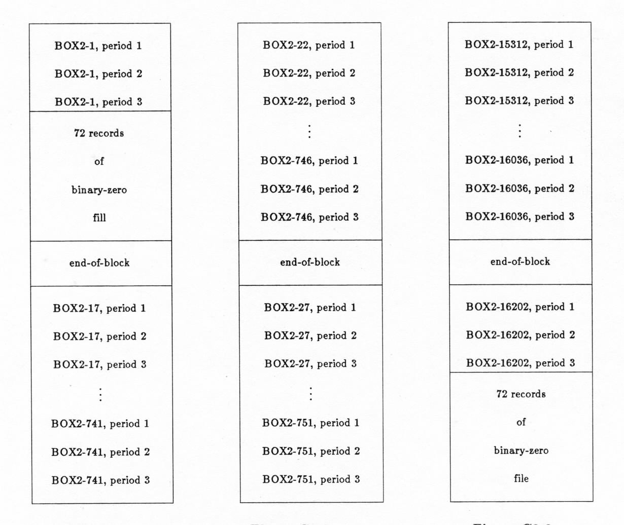
Figure C3-1 (left). BOX10-1 monthly structure.
Figure C3-2 (middle). BOX10-2 and -3 monthly structure (similar for BOX10-4 through -647).
Figure C3-3 (right). BOX10-648 monthly structure.
4. Trimming Performance (TRP)
This format gives detailed information, for each year-month-2° box and for each explicitly trimmed variable (S, A, U, V, P, and R), of the number of observations input, and the number trimmed for being above or below the limits provided by DSUL. Special configurations count the number of observations automatically rejected when no limits are provided or where a 2° box is landlocked. Thus a TRP was output if and only if a year-month-2° box contained at least one observation of one or more of the explicitly trimmed variables. Table C4-1a shows the bit layout of each TRP and Table C4-1b shows the bit layout of each of its 72-bit or 60-bit sections, in sequential bit-order reading from top to bottom.
 #  β    Statistic                             Bits
---------------------------------------------------
         rptin                                   16
         year                                     8
         month                                    4
         2° box                                  14
         10° box                                 10
         checksum                                12
---------------------------------------------------
19  ni   number of observations input            72
20  nl   number of observations lower-trimmed    60
21  nu   number of observations upper-trimmed    60
---------------------------------------------------
         total                                  256
 #  β   Variable                              Bits   Bits
---------------------------------------------------------
 1  S   sea surface temperature                 10     12
 2  A   air temperature                         10     12
 4  U   vector wind eastward component          10     12
 5  V   vector wind northward component         10     12
 6  P   sea level pressure                      10     12
 9  R   relative humidity                       10     12
---------------------------------------------------------
        total                                   60     72
The coded and true value ranges, the units, and the base of all these fields are common to the monthly summaries, with characteristics as given in sec. 2.3 of supp. A, except that the following fields have different names and other differences as noted:
These statistics have the same properties as n in the monthly summaries, except that the coded (and true value being the same) ranges are reduced to: 1≤4095 and 1≤1023 for the 12 and 10 bit fields, respectively.
For each of the univariates (S, A, P, R) the total number trimmed is nt = nl + nu and the number output is n = ni - nt (identical with n in the corresponding MST). For the bivariate [U V]' the total number trimmed is nt = nlU + nuU + nlV + nuV, where the notation αβ has its usual meaning, and niU = niV. In this case the order tests are made in gives a special meaning to the statistics for [U V]':
a) first, any observation with U < lU is counted by nlU,Either nl or nu (not both) greater than 0 in conjunction with ni 0 has a completely different meaning from that stated previously. Where the 2° box is landlocked, nl with ni 0 counts the number of observations input and automatically rejected. Otherwise, when no limits are provided, nu with ni 0 counts the number of observations input and automatically rejected. For [U V]' landlocked only nlU is set -- nuU, nlV, and nuV should be 0. Similarly, only nuU is set if the limits for U are missing, or only nuV is set if the limits for V are missing but those for U are not. These rules preserve the properties of the preceding equations for nt, if one desires to include in nt those observations landlocked or with missing limits.
b) any survivor of a) with U > uU is counted by nuU,
c) any survivor of b) with V < lV is counted by nlV,
d) any survivor of c) with V > uV is counted by nuV.