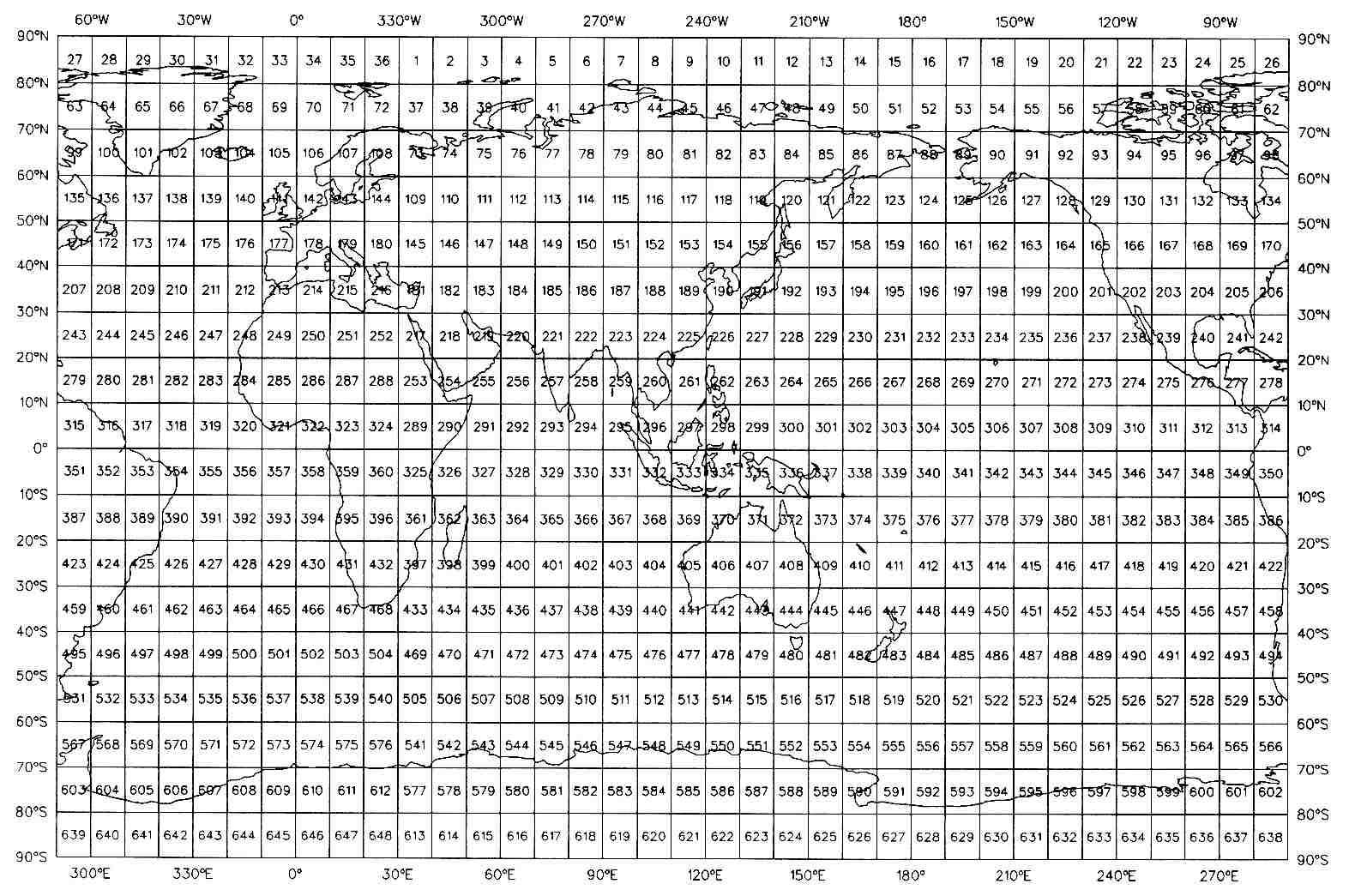
Figure 0-1. 10° box numbering system

CIRES  |  University of Colorado/NOAA
       |  Cooperative Institute for Research in Environmental Sciences
       |       Ralph J. Slutz
       |       Sandra J. Lubker
       |       Jane D. Hiscox
       |
ERL    |  U.S. Department of Commerce
       |  National Oceanic and Atmospheric Administration (NOAA)
       |  Environmental Research Laboratories
       |       Scott D. Woodruff
       |
NCAR   |  National Science Foundation sponsored
       |  National Center for Atmospheric Research
       |       Roy L. Jenne
       |       Dennis H. Joseph
       |
NCDC   |  U.S. Department of Commerce
       |  National Environmental Satellite, Data, and Information Service
       |  National Climatic Data Center
       |       Peter M. Steurer
       |       Joe D. Elms
Mention of a commercial company or product does not constitute an endorsement by NOAA/ERL. Use for publicity or advertising purposes, of information from this publication concerning proprietary products or the tests of such products, is not authorized.
This is an HTML Edition of this original publication:
Slutz, R.J., S.J. Lubker, J.D. Hiscox, S.D. Woodruff, R.L. Jenne, D.H. Joseph, P.M. Steurer, and J.D. Elms, 1985: Comprehensive Ocean-Atmosphere Data Set; Release 1. NOAA Environmental Research Laboratories, Climate Research Program, Boulder, CO, 268 pp. (NTIS PB86-105723).
Some changes in appearance or structure were made to facilitate rendering in HTML for navigation through the electronic version. Also a few minor errors or omissions in the original printed document were corrected, as noted within and marked in red.
An HTML-4.0 compatible browser is recommended for viewing the publication and its supplements. Note: This version of the document has not been fully proofread in comparison to the original printed edition, which should be referred to in the event of questions. Updated availability is from the Climate Diagnostics Center, NOAA, Boulder, Colorado, USA.
We express our appreciation to Bruce Bradshaw and Jean Gagnon of the Marine Environmental Data Service, and to Val Swail of the Meteorological Service, of Canada, for the scanned images received in 1998 on which much of this work was based. We are also grateful to Don Mock at the Climate Diagnostics Center for his extensive efforts to create this HTML edition.
Links to PDF files composing the original printed document (0.3MB to 4.8MB): MAIN | supp. A | supp. B | supp. C | supp. D | supp. E | supp. F | supp. G | supp. H | supp. I | supp. J | supp. K and to a tar file containing all the PDF files (19.5MB): release1_pdf.tar
To understand climate variability we must first delineate what kind of behavior must be understood. Do changes in the more energetic parts of the global climate machine occur gradually or suddenly? If there are clear "climate signals," where in the global domain do they appear first? How do they evolve in time? Do the signals reflected in various geophysical fields relate to one another in physically consistent ways? Do the forcing fields exhibit time variability that is consistent with the response fields? What does the behavior tell us about possible causes of climatic variability?
The opportunity to explore such questions has been severely limited by the availability of observations reflecting past behavior. Only since the advent of satellites have we been able to observe some few parameters on a global basis. Only since World War II have there been enough upper air observations to explore the vertical dimension and they are sparsely distributed. Only with surface observations can we extend the record of past behavior back into the last century.
In doing so, we find that the land stations having long records are too few to delineate spatial variability over the planet. Over the ocean areas, however, ship observations provide a richer record. They are good enough to delineate the time variability of the major wind systems and related fields of surface pressure and temperature.
The incentive for developing the Comprehensive Ocean-Atmosphere Data Set (COADS) was to make this record available to the individual investigator in a form that is reliable and easy to use. The global marine surface data set contains the most detailed record we will ever have of the dynamics of the global climate system over the last century and more. It should trigger rapid progress in understanding by making it possible to delineate the spatial and temporal characteristics of the several sharp adjustments of the global circulation that have occurred, and to glean from them clues to the nature and causes of global climate variability. COADS provides the material for diagnostic research to identify and explore the key questions. It also provides the needed boundary conditions for model simulation of the climate system variability.
It has taken four years and much effort by many individuals and several institutions to obtain and process the hundreds of tapes containing the basic data input. All of this effort was provided from ongoing activities; there was no appropriation identified for the task. It is a tribute to the spirit of cooperation among the participating organizations that the task has been successfully completed.
Throughout the effort, the support and encouragement of Dr. Wilmot N. Hess was crucial, as Director of ERL during the early stages and as Director of NCAR during the later stages.
Joseph O. Fletcher
J. Fletcher and U. Radok helped initiate and guide this project through the years; W. Hess at NCAR provided both computing resources and encouragement necessary to complete it. T. Potter provided essential support in the early stages. Many others contributed advice or assistance, among them: G. Caldwell, R. Cram, S. Esbenson, R. Keen, S. Khalsa, D. McLain, A. Oort, R. Quayle, C. Ramage, R. Reynolds, D. Shea, S. Warren, and B. Weare.
There would be no release without the programmers who have worked on it. Thanks to all of them including T. Brown, W. Otto, Y. Pann, T. Parker, J. Souder, W. Spangler, G. Walters, and X. Zhang. Thanks also to Martha Rife, because there would be no release without her invaluable typing.
The project has been cooperatively supported by funding from ERL, NCAR, and NCDC, with additional support from the Equatorial Pacific Ocean Climate Studies (EPOCS) program for the work by CIRES and ERL.
Global marine data observed during 1854-1979, primarily by ships-of-opportunity, have been collected, edited, and summarized statistically for each month of each year of the period, using 2° latitude x 2° longitude boxes. Products now available in a first release from this Comprehensive Ocean-Atmosphere Data Set (COADS) include fully quality-controlled (trimmed) reports and summaries. Each of the 70 million unique reports contains 28 elements of weather, position, etc., as well as flags indicating which observations were statistically trimmed. The summaries give 14 statistics, such as the median and mean, for each of eight observed variables of air and sea surface temperatures, wind, pressure, humidity, and cloudiness, plus 11 derived variables. Relatively noisy (untrimmed) individual reports and summaries (giving 14 statistics for each of the eight observed variables) are available for investigators who prefer their own quality control. Two other report forms, inventories, and decade-month summaries are among the other data products available. FORTRAN 77 software available to help read "packed binary" data products and processing details, such as the method of identifying duplicate reports, are also described.
Since 1854, ships of many countries have been taking regular observations of local weather, sea surface temperature, and many other characteristics near the boundary between the ocean and the atmosphere. The observations by one such ship-of-opportunity at one time and place, usually incidental to its voyage, make up a marine report. In later years fixed research vessels, buoys, and other devices have contributed data. Marine reports have been collected, often in machine-readable form, by various agencies and countries. That vast collection of data, spanning the global oceans from the mid-nineteenth century to date, is the historical ocean-atmosphere record.
The aim of this project was to assemble and reduce machine-readable portions of the available historical ocean-atmosphere record into a regular, compact, easily-used data base at three principal resolutions: 1) individual reports, 2) year-month summaries of the individual reports in 2° latitude x 2° longitude boxes, and 3) decade-month summaries. Duplicate reports judged inferior by a first quality control process designed by the National Climatic Data Center (NCDC) were eliminated or flagged, and "untrimmed" monthly and decadal summaries were computed for acceptable data within each 2° latitude x 2° longitude box. Tighter, median-smoothed limits were used as criteria for statistical rejection of apparent outliers from the data used for separate sets of "trimmed" monthly and decadal summaries. Individual observations were retained in report form but flagged during this second quality control process if they fell outside 2.8 or 3.5 (trimmed from statistics) estimated standard-deviations about the smoothed median applicable to their 2° latitude x 2° longitude box, month, and 56-, 40-, or 30- year period (i.e., 1854-1909, 1910-1949, or 1950-1979).
Eight "observed" variables were included in the untrimmed monthly summaries:
     1    S    sea surface temperature
     2    A    air temperature
     3    W    scalar wind
     4    U    vector wind eastward component
     5    V    vector wind northward component
     6    P    sea level pressure
     7    C    total cloudiness
     8    Q    specific humidity
Included in the trimmed monthly summaries were the eight observed
variables plus 11 derived variables:
     9    R    relative humidity
     10   D    S - A = sea-air temperature difference
     11   E    (S - A)W = sea-air temperature difference * wind magnitude
     12   F    Qs - Q = (saturation Q at S) - Q
     13   G    FW = (Qs - Q)W (evaporation parameter)
     14   X    WU
     15   Y    WV (14-15 are wind stress parameters)
     16   I    UA
     17   J    VA
     18   K    UQ
     19   L    VQ (16-19 are sensible and latent heat transport parameters)
For each variable, 14 statistics were computed:
     1    d    mean day-of-month of observations
     2    h    hour statistic
     3    x    mean longitude of observations
     4    y    mean latitude of observations
     5    n    number of observations
     6    m    mean
     7    s    standard deviation
     8    0    0/6 sextile (the minimum)
     9    1    1/6 sextile (a robust estimate of m - 1s)
     10   2    2/6 sextile
     11   3    3/6 sextile (the median)
     12   4    4/6 sextile
     13   5    5/6 sextile (a robust estimate of m + 1s)
     14   6    6/6 sextile (the maximum)
All the other historical observations, such as present and past
weather, visibility, and waves, are available in report form.
This report gives an overall description of the workplan, indicating products available in this first release of the Comprehensive Ocean-Atmosphere Data Set (COADS). Sources of the data, some characteristics of their distribution in time and space, and cautions in using them are also included. Product formats, software listings, processing details, and background material are presented in supplements A-K to this report. A number enclosed in brackets refers to references, e.g., [1].
Release 1 of COADS offers 14 data products; 13 available from the National Center for Atmospheric Research (NCAR), and one available from NCDC. Because of the volume of data and for reasons of computational efficiency, all but the NCDC product are stored in "packed binary" formats, whereby data were coded as positive integers and the resultant binary bit-strings were packed into bytes of the smallest convenient length. Reconstruction of floating-point data requires that the byte length and two other characteristics of each field be externally specified. Machine-transportable* FORTRAN 77 software that includes these specifications is available in addition to the data products (see supp. H).
Global systems of numbering 10° latitude x 10° longitude and 2° latitude x 2° longitude boxes** were also developed with the efficient and convenient storage of data in mind. Figure 0-1 illustrates the 10° box system, which has box numbers spiraling eastward down from number 1, with its lower-left (SW) corner at 30°E, 80°N, to number 648 at 20°E, 90°S. The 30°E division was chosen to avoid splitting any ocean, which facilitates the retrieval of latitude bands of data stored in box-order on serial media (such as magnetic tape). The 2° box system is similar, and these and other location systems, such as the historic system of Marsden Squares still used by NCDC, are described in detail in supp. G.
Figure 0-1. 10° box numbering system
Any conclusion drawn from the historical record should be qualified by the fact that the observation, reporting, collection, and digitization of these data have been subject to a great deal of methodological change. Besides introducing more or less unknown inhomogeneities into many variables, these changes have sometimes been processed incorrectly. The resulting errors, as well as simple recording or transmission errors, occur very frequently. While a major effort has been made to indicate reports containing errors, some kinds of errors cannot be trapped by statistical methods. A very common error in the original data was incorrect representation of latitude and longitude, and only in extreme cases were these identified. Thus it must be remembered that while millions of errors have been identified and eliminated from the trimmed summaries, the resulting data are still far from clean. In addition, the distribution of data is highly variable in both time and space. Nevertheless, such a unique and clearly irreplaceable historical record is worthy of exhaustive study on the scale of either weather or climate, provided it is used with careful attention to these characteristics (see sec. 4 for more information).
The period of record is 1854 through 1979;*** a few reports found in these data before 1854 are thought to have spurious times digitized and were excluded at later stages of processing. Owing to erroneous latitudes and longitudes, a significant amount of data also falls on land, increasing dramatically with the advent of global telecommunications (c. 1966). However, the increase is only partly real, because some inputs for earlier years had the land data deleted (see sec. 3). Reports for approximate land locations were also flagged or excluded at later stages of processing.
COADS Release 1 is the culmination of four years of cooperation
among the Cooperative Institute for Research in Environmental Sciences
(CIRES), the Environmental Research Laboratories (ERL), and NCDC,
joined in the last three years by NCAR. In addition to specifying
requirements for the initial quality control and duplicate elimination
process, and checking their proper implementation, NCDC was
responsible for acquiring the bulk of the data. Programs for
conversion of individual marine reports back and forth from characters
to binary, sorting, input/output, and other tasks were written and
executed by NCAR staff; quality control, duplicate elimination,
reformatting, calculation of monthly and decadal summaries, and
trimming were among those accomplished by CIRES and ERL staff. Except
for testing and auxiliary steps, processing was accomplished on NCAR
computers, especially their previous CDC 7600 and current Cray 1,
requiring over 100 hours of Cray-equivalent CPU time.
_____________________
* Machine-transportable software may require changes to work on
different computer systems (given certain minimum machine
requirements), but these modifications are few and well defined.
** The notation BOXn (e.g., BOX2 or BOX10) will be used to denote
an n° latitude x n° longitude box, or more simply, n° box.
*** An update through 1984 of selected products is planned for
availability in 1987.
_____________________
1. Data Input
An attempt was made to integrate all available, digitized,
directly sensed surface-marine data sets that would contribute
information of reasonable quality, so that the final set would be as
comprehensive as possible. The data sets listed in Table 1-1 were
collected and input to the first stages of processing; details on each
data set can be found in supp. K. An original goal
of the project was to update the Atlas data set used by NCDC to construct a
set of marine atlases, e.g., [11],
using data from the Historical Sea Surface Temperature (HSST) Data Project.
The 1854-1969 period of the Atlas was extended through 1979 using NCDC's '70s
Decade data set, and other additions to later years such as buoy,
bathythermograph, and IMMPC (International Exchange) data. Other data were
included because of their high quality (Ocean Station Vessels) or remote
location (South African Whaling). The data sets listed in Table 1-2 were
left out for one reason or another; in addition to these, the final data set
includes no remotely sensed data.
                               Million reports (approx.)           Source
-------------------------------------------------------------------------
Atlas                                   38.6                         NCDC
HSST (Historical Sea Surface
   Temperature Data Project)            25.2                NCDC, Germany
Old TDF - 11 Supplements B and C         7                           NCDC
Monterey Telecommunication               4                           NCDC
Ocean Station Vessels, and Supplement    0.9                         NCDC
Marsden Square 486 Pre-1940              0.07                        NCDC
Marsden Square 105 Post-1928             0.1                         NCDC
National Oceanographic Data Center
   (NODC) Surface, and Supplement        2                           NCDC
Australian Ship Data (file 1)            0.2                    Australia
Japanese Ship Data                       0.13                      M.I.T.
IMMPC (International Exchange)           3                           NCDC
South African Whaling                    0.1                         NCAR
Eltanin                                  0.001                       NCDC
'70s Decade                             18                           NCDC
IMMPC (International Exchange)*          0.9                         NCDC
Ocean Station Vessel Z*                  0.004                       NCDC
Australian Ship Data (file 2)*           0.2                    Australia
Buoy Data*                               0.3                         NCDC
'70s Decade Mislocated Data*             0.003                       NCDC
                                       -------
                                       100**
-------------------------------------------------------------------------

* Additions solely to 1970-1979 decade.
** The approximate total includes 26.58 million relatively certain
duplicates, and some seriously defective or mis-sorted reports, which
were removed by initial processing steps.
__________________
                                          Million reports (approx.)    Source
-----------------------------------------------------------------------------
Ocean Station Vessel Upgrade (TD-1160)*              1.71                NCDC
Islas Orcadas (Eltanin)                              ?              Argentina
FCDS (Fleet Consolidated Data Set)**                20              U.S. Navy
New Navy GTS (Global Telecommunication System)*      ?              U.S. Navy
British Marine Data Bank**                          40         United Kingdom
TD-1117 U.S. Navy Hourlies (a few were included)     ?                   NCDC
TD-13SY                                              ?                   NCAR
TD-1393 Pickets                                      ?                   NCAR
TD-1313 Marine                                       ?                   NCAR
National Meteorological Center Data (NMC)*           ?               NOAA/NMC
-----------------------------------------------------------------------------

* Many of these data were included from OSV or GTS data (e.g., from U.S. Air
Force Global Weather Central) within sources listed in Table 1-1.
** It is thought that most of these data were included within sources listed
in Table 1-1.
___________________
The overall workplan is shown jointly by Flowchart 1 (primary processing) and Flowchart 2 (secondary processing). All steps are completed, but five of the nineteen data products are not available because they have been superseded by other products as noted.
The 14 data products that are available for distribution (see secs. 2.1.1 and 2.2.1) are marked "(Avail.)." Currently, the 13 of these products that are recorded in packed binary formats can be obtained on magnetic tape from the
(Basic sets of reports and statistics, as updated, will be available indefinitely; minor products may later be reviewed for retention.) Descriptions of the available products and some of the other products and processes shown will be found in supps. A-K. See supp. H for listings of FORTRAN 77 software that may assist users in reading packed binary data products; these programs are also available at NCAR on magnetic tape.
Even though packed binary methods were employed to store all but one (product 19; TD-1129) of the 14 available data products, some of them are still very voluminous. This is because of the diversity of observed and statistical information, and the wide coverage and fine resolution in both space and time. For users not needing complete data products, copies can usually be made for selected areas or times by NCAR or NCDC.
Since the 1970-1979 decade was processed separately throughout the initial work, separate '70s and pre-'70s files are provided for individual marine reports and other initial products (as noted in each product description in secs. 2.1.1 and 2.2.1). Depending on the application, this may or may not be a convenience to the user. An effort was made to integrate the two periods in all the final monthly summaries and other products of later stages of processing, as well as to remove data before 1854. Data over land were also removed only at later stages. This provides a measure of positional noise to be expected in supposedly legitimate samples. Supp. G shows approximately which 2° boxes are over land; a machine-readable world map showing the land boxes is available at NCAR, and was used in deleting "landlocked" data.

Flowchart 1. Primary Processing. Data products are shown as circles and
processes are shown as squares. (Note: product 3 has been superseded by
product 10, and products 4, 5, and 7 have been superseded by secondary
products 12-18 shown on Flowchart 2.)
2.1 Primary Processing: Flowchart 1
The primary processing yielded all of the basic products, but left them in a form that is difficult for the average user to cope with because of size, ordering, and complexity. (The secondary processing seeks to manipulate these into more user-friendly arrangements.) The basic goals of the primary processing were as follows.
1) To compact and modernize the representation and ordering of individual marine reports without loss of information. For a database of this size, traditional character-based representations are extremely wasteful in both storage and processing costs. Conversion to a packed binary representation (process a on Flowchart 1) based on storing positive integers in minimal-length strings of bits was used to halve storage size (product 1 on Flowchart 1). This format was computationally efficient for the processes (b-c) of sorting, quality control, and the elimination of more than one-fourth of the reports as "certain" duplicates. Inventories (product 2) describe the distribution of reports in time and space and their source. The most commonly used portions of each unique report were also re-expressed in an extremely compact form (product 3), with flags added later (product 10) to indicate which observations failed the second (trimming) stage of quality control.
2) To summarize different variables on a monthly scale in 2° boxes, producing traditional and robust statistics for the expected value and standard deviation, as well as centroids of observational location in time and space. A first set of "untrimmed" statistics (product 4) summarizes observed variables after using flags from the initial quality control to reject gross errors, but before any further quality control (with the untrimmed statistics, or by ignoring the flags on individual observations in product 10, users retain the freedom of applying their own additional quality control). A second set of "trimmed" statistics (product 7) summarizes observed plus derived variables after further quality control to remove apparent statistical outliers. Trimming performance data (product 8) count observations trimmed from each 2° box and month.
3) In parallel with the monthly summaries, to summarize trimmed and untrimmed data on a decade-month scale in 2° boxes. Decadal summaries (products 5 and 9) may not be the "best" representatives of a decade, because of temporal inhomogeneity, but they contain statistics (such as the true decadal median) that cannot be generated from the monthly summaries. Smoothed aggregates of the untrimmed decadal summaries (product 6) were used for limits on which to perform the trimming.
The processes used to meet these goals and the products that result are shown in Flowchart 1, and described individually as follows. All the primary products are stored in packed binary formats, except that product 1 (Long Marine Reports) has a hybrid format consisting of packed binary plus characters.
2.1.1 Primary Products (Flowchart 1)
Product 1. (Avail.) Long Marine Reports (LMR*).This is the format for individual reports output from processes a through c. LMR contain the complete observational record, including quality flags, illegal characters, and supplemental fields, stored in a variable-length format (refer to supp. F) averaging one-half the size of the less complete 148 (8-bit) character NCDC result (TD-1129). Sort is by 10° box, year, month, 1° box, day, hour, and card deck, and possible duplicates have either been eliminated or flagged. Coverage: 1800-1969, 1970-1979 separately; landlocked reports are flagged.
Product 2. (Avail.) Inventories (INV).Includes the number of individual LMR in each year-month and 10° box, as well as summary information giving (approximate) quality-control flag counts and the makeup of each 10° box by card deck and source (supp. K). Sort is by 10° box. Coverage: 1800-1969, 1970-1979 separately; landlocked reports are included.
Product 3. Compressed Marine Reports (CMR.4).This format for individual reports contains 29 frequently used elements (see supp. E). Sort is by 10° box, month, 2° box, year, day, hour, longitude, latitude. Coverage: 1800-1969, 1970-1979 separately; landlocked reports are included. It has been superseded by product 10.
Product 4. Monthly Summaries Untrimmed (MSU.1).Eight observed variables, each described by 14 statistics for 2° boxes. Sort is by 10° box, month, 2° box, year. Coverage: 1800-1969, 1970-1979 separately; landlocked data are included. Secondary products 13, 14, and 17 are available instead.
Product 5. Decadal Summaries Untrimmed (DSU.1).Input to the smoothing process used to create the statistical basis for trimming outliers (product 6). Sort is by 10° box, month, 2° box, decade. Coverage: 1800-1969, 1970-1979 separately; landlocked data are included. It has been superseded by product 12.
Product 6. (Avail.) Decadal Summary Untrimmed Limits (DSUL).Possibly asymmetric upper and lower limits about a smoothed median were constructed from product 5 (supp. C) and used later to trim outliers from three periods (1854-1909, 1910-1949, and 1950-1979). Sort is by 10° box, month, 2° box, period. Coverage: 1854-1979; landlocked 2° boxes are flagged.
Product 7. Monthly Summaries Trimmed (MST).Nineteen observed and derived variables, each described by 14 statistics for 2° boxes (supp. A). Sort is by 10° box, month, 2° box, year. Coverage: 1854-1969, 1970-1979 separately; landlocked data are deleted. Secondary products 15, 16, and 18 are available instead.
Product 8. (Avail.) Trimming Performance (TRP).Gives information (see supp. C) for each 2° box and year-month of the number of explicitly trimmed variables found to be above or below the limits set by DSUL. Sort is by 10° box, 2° box, year, month. Coverage: 1854-1979; landlocked data are counted.
Product 9. (Avail.) Decadal Summaries Trimmed (DST).Seven variables, each described by 10 statistics (plus sums of squares and cross products of vector wind) for 2° boxes, with the format as given in supp. A. Sort is by 10° box, month, 2° box, decade. Coverage: 1854-1969, 1970-1979 separately; landlocked data are deleted.
Product 10. (Avail.) Compressed Marine Reports (CMR.5).This format for individual reports contains 28 frequently used elements, and supersedes product 3 as an extremely compact alternative to LMR. Individual ship number or call sign is omitted, as are wave and swell fields, etc. During statistics pass 2 (process g), variables outside 2.8 or 3.5 (trimmed from statistics) estimated standard-deviations about a smoothed median were retained but flagged in a fixed-length format (shown in supp. D) totaling one-sixth the size of the 148 (8-bit) character NCDC result (product 19). Sort is by 10° box, month, 2° box, year, day, hour, longitude, latitude. Coverage: 1854-1969, 1970-1979 separately; landlocked reports are flagged.
2.1.2 Primary Processes (Flowchart 1)
Process b. Sort
Input data as received were sorted in many different ways. This
step sorted all data into the sequence necessary for duplicate
elimination (10° box, year, month, 1° box, day, hour, and card
deck).
Process c. QC/dupelim
The data were first quality controlled, and the resulting flags
used to select the best report in the event of duplicates.
Duplicate elimination was complicated by the fact that duplicates
were frequently found across hours or days. These steps were
coded according to NCDC specifications as shown by
supp. J and supp. K.
Process d. Convert and Sort
This converted LMR into CMR.4; supp. E contains
translation details. The sort required by the statistics programs has
"month" as the first key after "10° box" in order that monthly and
decadal statistics could be generated simultaneously.
Process e. Statistics Pass 1
Using as input CMR.4, this produced both 2° monthly and decadal
statistics (refer to supp. A,
supp. B, and supp. C).
Process f. Smooth
DSU.1 resulting from Pass 1 were smoothed in order to provide
limits for trimming. Line-printer plotting and hand analysis of
areas such as coastlines were required to ensure proper smoothing
(see supp. C).
Process g. Statistics Pass 2
Using as input CMR.4 and DSUL, this produced trimmed 2° monthly
and decadal summaries, plus CMR.5 for those who wish to compute
their own statistics using a clean observation set.
Supp. A, supp. B, and
supp. C show computational details.
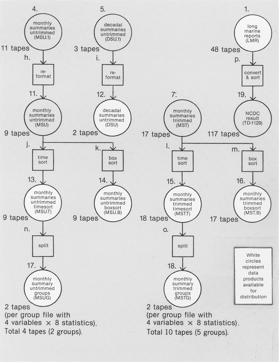
Flowchart 2. Secondary Processing. Data products are shown as circles and
processes are shown as squares.
2.2 Secondary Processing: Flowchart 2
The products from the primary processing were individual reports, decadal summaries, and monthly summaries in a sort by 10° box, month, 2° box, year. This sort is acceptable for analyses in limited areas, but is inconvenient and costly when used for delineating global conditions at specific times. Similarly, the files at this stage contain many different statistics and climate variables in each record, and most analyses use only a few quantities at a time. Therefore, additional work was needed to make the data economical to access, and to bring the entire matrix of monthly summary output, over 9.2 billion pieces of information on 26 6250-cpi tapes, within easy reach of the individual investigator. Procedures were as follows.
1) The monthly summaries were sorted into the "timesort" of products 13 and 15 shown on Flowchart 2. The time (or synoptic) sort, by pure time (January 1855 follows December 1854, etc.) and then 2° box, permits analysis of the globe at each time step, in sequence. A "boxsort", by 2° box and then pure time within each 10° box, was completed (products 14 and 16) for studies that concentrate on a small area. The untrimmed monthly and decadal summaries also were reformatted in order to make the formats of products 11 and 12 compatible with their trimmed counterparts, and to achieve a significant (about 15%) reduction in size.
2) The monthly summaries in timesort were separated into group files so it would not be necessary to pass over unwanted data. Typically, studies will require grouping mean-estimates of a variable together with the number of observations, a standard deviation estimate, and centroids of observational location in time and space, so that smoothed grids might be generated taking into account all the different aspects of variability. The group files combine four such variable-ensembles, and serve as the primary exchange format (products 17 and 18). For some selected values of very common use, such as the mean of sea surface temperature, individual files may later be generated.
3) With major work by NCAR the individual reports were converted into NCDC's standard character format (product 19). Because of the large computing requirements, it was important that the very complex transformation be properly generated. Therefore, sample tapes were sent to NCDC to be checked.
Flowchart 2 shows the secondary products and processes, as described individually in the following. All the secondary products are stored in packed binary formats, except that product 19 (TD-1129) has an ordinary character format.
2.2.1 Secondary Products (Flowchart 2)
Product 11. Monthly Summaries Untrimmed (MSU).Eight observed variables, each described by 14 statistics for 2° boxes, with the format as given in supp. A (this carries essentially the same information as product 4, but in a more efficient format compatible with that of its trimmed counterpart, product 7). Sort is by 10° box, month, 2° box, year. Coverage: 1854-1969, 1970-1979 separately; landlocked data are included. Products 13, 14, and 17 are available instead.
Product 12. (Avail.) Decadal Summaries Untrimmed (DSU).Six variables, each described by eight statistics (plus sums of squares and cross products of vector wind) for 2° boxes, with the format as given in supp. A (this carries essentially the same information as product 5, but in a more efficient format similar to that of its trimmed counterpart, product 9). Sort is by 10° box, month, 2° box, decade. Coverage: 1854-1969, 1970-1979 separately; landlocked data are included.
Product 13. (Avail.) Monthly Summaries Untrimmed Timesort (MSU.T).Eight observed variables, each described by 14 statistics for 2° boxes, with the format as given in supp. A. Sort is by year, month, 2° box (also called synoptic sort). Coverage: 1854-1979; landlocked data are included.
Product 14. (Avail.) Monthly Summaries Untrimmed Boxsort (MSU.B).This is product 13, sorted instead by 10° box, 2° box, year, month. Coverage: 1854-1979; landlocked data are included.
Product 15. (Avail.) Monthly Summaries Trimmed Timesort (MST.T).Nineteen observed and derived variables, each described by 14 statistics for 2° boxes, with the format as given in supp. A. Sort is by year, month, 2° box (also called synoptic sort). Coverage: 1854-1979; landlocked data are deleted.
Product 16. (Avail.) Monthly Summaries Trimmed Boxsort (MST.B).This is product 15, sorted instead by 10° box, 2° box, year, month. Coverage: 1854-1979; landlocked data are deleted.
Product 17. (Avail.) Monthly Summary Untrimmed Groups (MSUG) andThese files (described in supp. B) are intended as a manageable alternative to the timesort files, in terms of processing and storage costs, for studies using only a few variables and statistics. Sort is by year, month, 2° box (also called synoptic sort). Coverage: 1854-1979; landlocked data are deleted.
Product 18. (Avail.) Monthly Summary Trimmed Groups (MSTG).
The two untrimmed groups (numbered 1-2) and the five trimmed groups (numbered 3-7) each contain four variables, with eight statistics included for each variable. For example, group 3 contains these statistics:
Product 19. (Avail.) NCDC Result (TD-1129).A subset of the full observational record in LMR is now available for distribution by NCDC in its TD-1129 ascii-character format. This is a 148-character format (see supp. I) sorted by Marsden Square, year, month, 1° Marsden Square, day, hour, card deck. (NCDC plans to re-sort this by Marsden Square, 1° Marsden Square, year, month, day, hour.) Coverage: 1800-1969, 1970-1979 separately; landlocked data are flagged.
2.2.2 Secondary Processes (Flowchart 2)
Processes j. and l. Time Sort
The monthly summaries were sorted by year-month and then 2° box.
Processes k. and m. Box Sort
The monthly summaries were sorted by 2° box and then year-month,
within each 10° box. Contrast this with the sort of products 7 and 11.
Processes n. and o. Split
The complete monthly summary matrices (untrimmed 8 variables x 14
statistics, trimmed 19 variables x 14 statistics) were split up
into group files (4 variables x 8 statistics). In this process,
the centroids of time/space location were shortened in length and
precision (as given in supp. B).
Process p. Convert and Sort
This converts LMR back to TD-1129 for NCDC. A sort is required in
order to change the first key from "10° box" to "Marsden
Square."
Results here show characteristics of the data at various stages, primarily after process c (QC/dupelim). Except for the summaries output from process g (statistics pass 2) and their derivatives, these results also include substantial amounts of data over land that were removed only at later stages of processing. For example, only two 10° boxes in the 1970s have no apparent data.
Table 3-1a lists the number of product records output from various processes; Tables 3-1b and 3-1c give related percentages. The precise definition of "certain" and "uncertain" duplicates (dups) is given by supp. K -- but it will suffice at this stage to allude to the degree of certainty in correctly identifying dups, with the "uncertain" being retained with flags in the LMR output, and removed from the TD-1129. The 1970s output is tabulated separately in each case, even if it was not run separately.
    Process                Output          Pre-'70s      '70s       Total
-----------------------------------------------------------------------------
b.a sort             LMR                  74,633,905  23,817,437  98,451,342b
c. QC/dupelim        1.a LMR (total)      53,185,975  18,682,484  71,868,459
                     1.  LMR (uncertain)     329,233      57,825     387,058
g. statistics pass 2 8.  TRP               3,699,340     833,847   4,533,187
                     9.  DST                 765,745c    102,463c    868,208c
                     10. CMR.5            52,840,447  18,622,039  71,462,486
i. reformat          12. DSU                 776,543     128,122     904,665
j. time sort         13. MSU.T             3,680,781     788,866   4,469,647
k. box sort          14. MSU.B             3,680,781     788,866   4,469,647
l. time sort         15. MST.T             3,685,123c    785,223c  4,470,346c
m. box sort          16. MST.B             3,685,123     785,223   4,470,346
n. split             17. MSUG (each group) 3,680,781     788,866   4,469,647
o. split             18. MSTG (each group) 3,685,123     785,223   4,470,346
p. convert and sort  19. TD-1129          52,856,742  18,624,659  71,481,401
-----------------------------------------------------------------------------

a Letters and numbers refer to Flowcharts 1 and 2 (LMR output from process b
was an intermediate product).
b The discrepancy between the total from process b and that given in Table
1-1 is largely because of the removal of seriously defective or mis-sorted
reports prior to this stage.
c It is thought that deletion of land data mainly accounts for the drop in
the number of DST in comparison to DSU, but that inclusion of Monterey
Telecom. (card deck 555) data only in the trimmed summaries more or less
compensates for this effect in the number of MST in comparison to MSU.
Supp. A has details on these and other criteria governing summary output.
____________________
Percentage of process output                     Pre-'70s  '70s   Total
-----------------------------------------------------------------------
percentage of b duplicate (certain + uncertain)     29      22      27
percentage of c uncertain                            1       0.3     1
-----------------------------------------------------------------------
Source*   Pre-'70s       '70s        Total
          b  c           b  c        b   c
--------------------------------------------
GTS       3  3           37 46       11  14
non-GTS   97 97          63 54       89  86
Buoy      0  0           2  2        1   0.5
IMMPC     21 25          58 50       30  32
NODC      2  3           1  2        2   2
HSST      34 16          0  0        26  12
--------------------------------------------

* Global telecommunication system (GTS) data
were identified by card deck (see supp. F):
555, 666, 849, 850, 888, 889, 999. Non-GTS
data comprise all other card decks, as well
as identifiable data from the remaining cat-
egories: buoy decks 143, 876-882; IMMPC 128,
926-928; NODC 891; and HSST 150-156.
___________________
The highest curve in Figure 3-7 is like that of Figure 3-1, but shows global reports per year rather than per month. Underneath are two curves of global reports per year input to dupelim: 1) from NCDC's Atlas data set, extended for 1970-1979 using their '70s Decade data set and 2) from the HSST data set. These three data sets are the largest inputs to COADS, and significant data sets scientifically.
Figure 3-8 (p. 25) is a map showing, for each 10° box, the log10 of reports output from dupelim, summed for all months from 1854 through 1979. The log10 is blank only for a box containing no data whatsoever, i.e., box 638. Figures 3-9 through 3-21 are similar maps for decades (starting with the fractional decade 1854-1859, then 1860-1869, etc.). Note the increase through time of data over land, especially for the 1960s and 1970s. This is coincident with when the global telecommunication system (GTS) starts, but is at least partly an artifact of previous editing procedures that removed earlier land data.

Figure 3-1. Global reports after duplicate elimination.
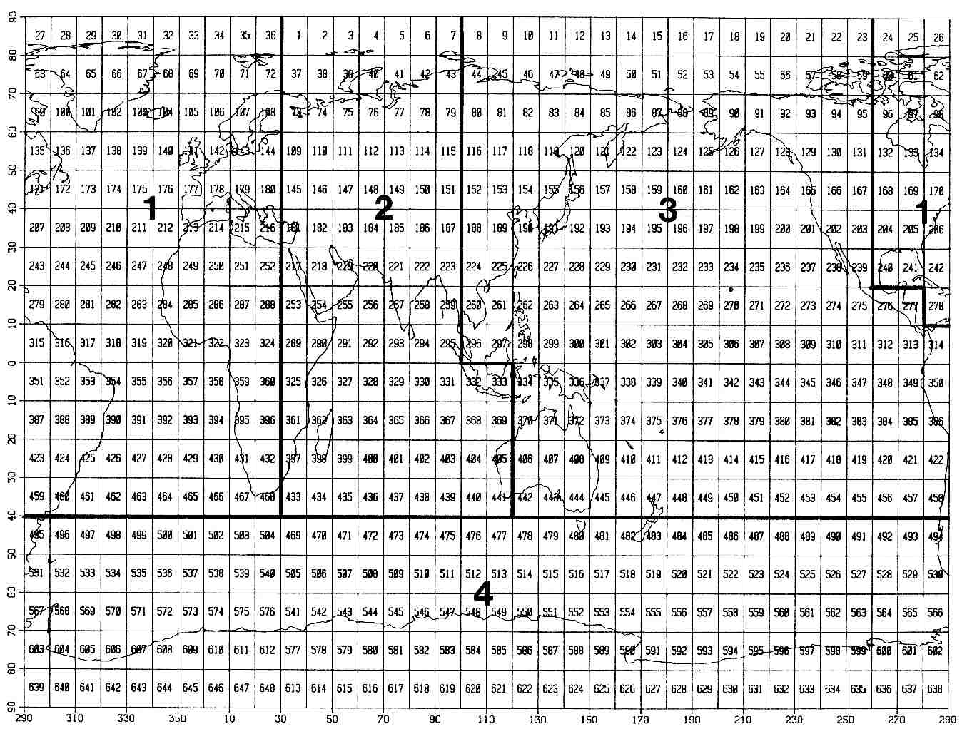
Figure 3-2. Basins and 10° boxes.
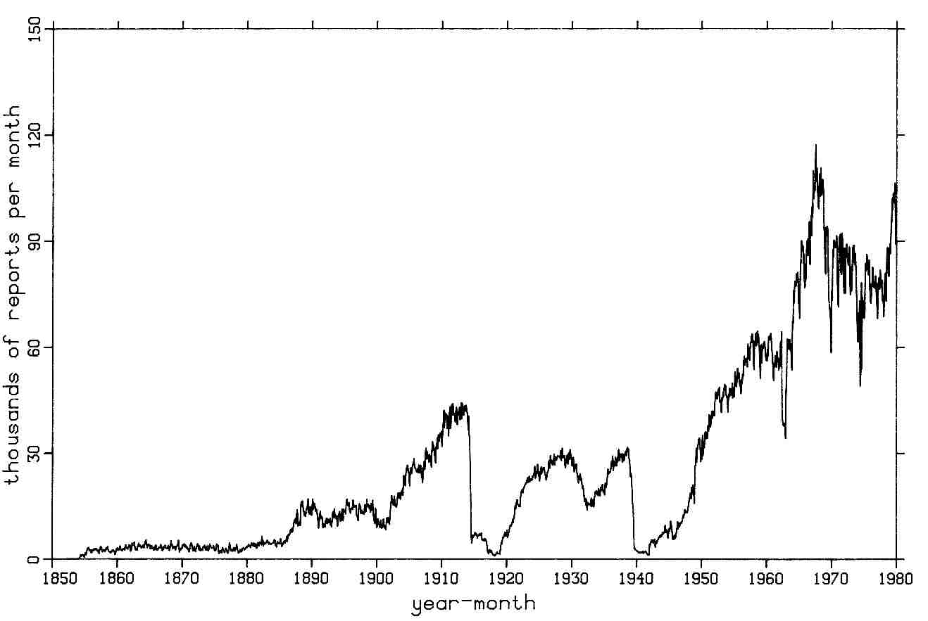
Figure 3-3. Basin 1 ATLANTIC reports after duplicate elimination.
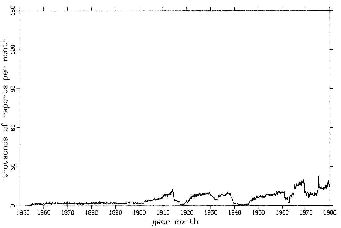
Figure 3-4. Basin 2 INDIAN reports after duplicate elimination.
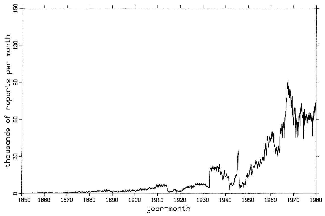
Figure 3-5. Basin 3 PACIFIC reports after duplicate elimination.
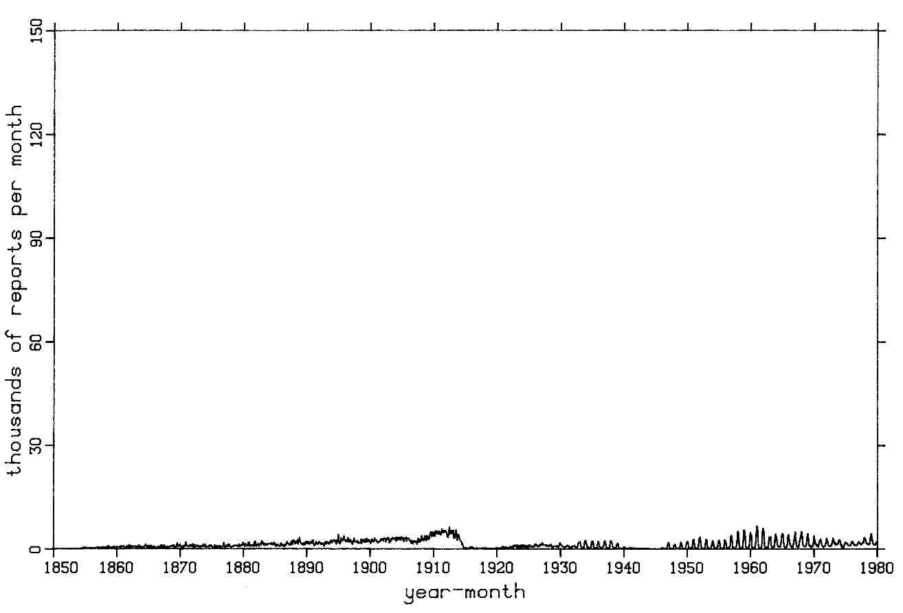
Figure 3-6. Basin 4 ANTARCTIC reports after duplicate elimination.
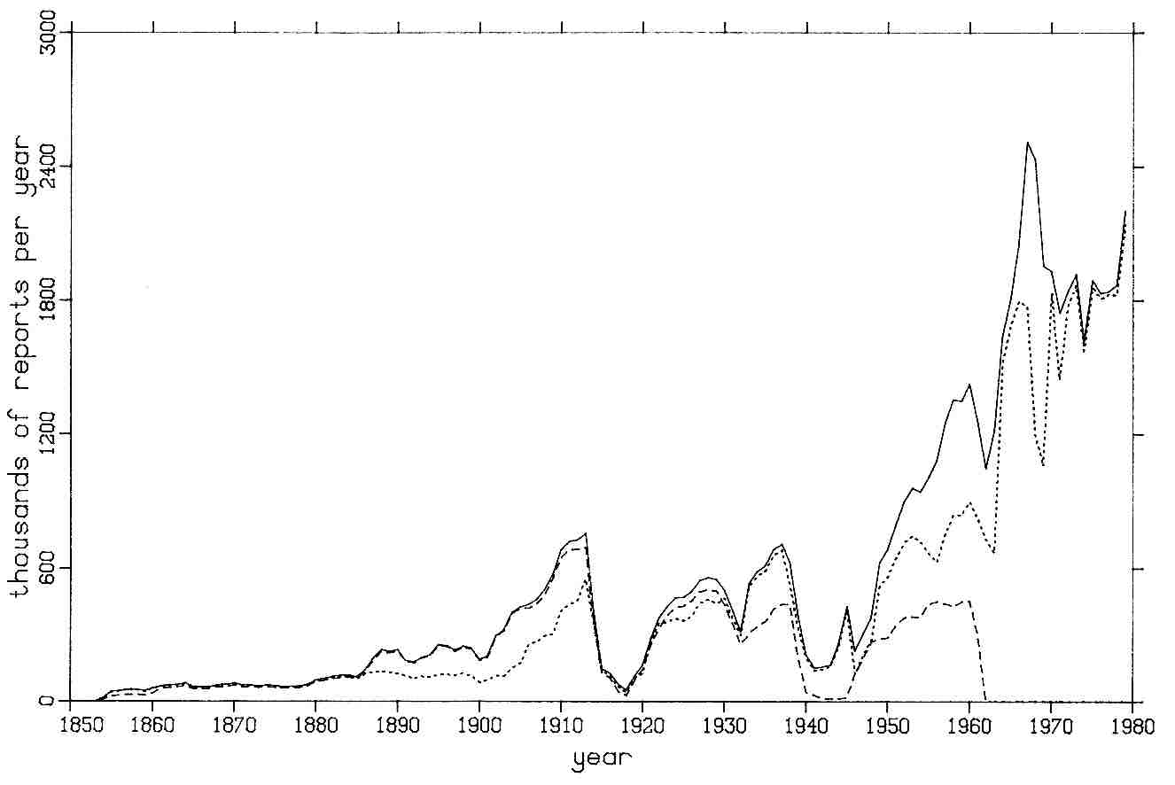
Figure 3-7. Annual global reports after duplicate elimination (solid); Atlas input (dotted, through 1969) continued by '70s Decade (dotted, 1970-1979); and HSST input (dashed, through 1961).
Table 3-2 is a frequency distribution of the number of untrimmed
monthly summaries (i.e., year-month-2° boxes) having different
counts of sea surface temperature observations for statistics. These
are given for four different 10° boxes (see Figure 3-2), for the '70s
decade. As one goes back in time, more of the boxes will have fewer
observations.
-------------------------------------------------------------------------------
Observations |                           10° box
          of |-----------------------------------------------------------------
 sea surface |       163             176             420             438
 temperature |(Gulf of Alaska) (Spanish Coast)   (N. Chile)   (S. Indian Ocean)
-------------|-----------------------------------------------------------------
           1 |         3               1             553             745
           2 |        14               3             210             553
           3 |        20               8              76             336
           4 |        41               2              33             216
           5 |        49              10              18             157
           6 |        61              14               7              81
           7 |        96              21               3              62
           8 |        96              15               3              39
           9 |       101              19               3              30
       10-99 |      2519            2349               1              39
     100-999 |         0             557               0               0
        >999 |         0               0               0               0
-------------------------------------------------------------------------------
                               Period     S      A   U and V   P      R
--------------------------------------------------------------------------
input (million observations) pre-'70s   47.19  50.15  50.88  37.09  23.09
                                 '70s   16.06  17.90  17.79  17.55  13.59
                                total   63.25  68.05  68.67  54.65  36.68

percentage trimmed           pre-'70s    1.24   0.92   1.61   0.65   0.26*
                                 '70s    2.28   1.46   1.39   0.92   0.43
                                total    1.51   1.06   1.56   0.74   0.32

percentage mislocated (est.) pre-'70s    0.05   0.07   0.09   0.12   n/a
                                 '70s    1.21   1.26   1.28   1.28   n/a
                                total    0.35   0.38   0.40   0.49   n/a
--------------------------------------------------------------------------

* One condition required before relative humidity R could be computed
was that air temperature A not be trimmed; this is the percentage of R
(only) trimmed afterwards.
___________________
                      Record length          Block size   60-bit   64-bit    Record
Gbita   Tapes Product    (bits)     Blocked    (bits)     words    words      count
-------------------------------------------------------------------------------------
39.5     48   1. LMR       549b      169c     64,000c    1,066.7  1,000   71,868,459
 0.089    1   2. INV    69,294b        1     198,240c    3,304    3,097.5      1,285d
13.7     17e  3. CMR.4     192       150      28,800       480      450   71,462,542
 8.58    11e  4. MSU.1   1,920        15      28,800       480      450    4,469,669
 0.868    3   5. DSU.1     960        30      28,800       480      450      904,687
 0.224    1   6. DSUL      384        75      28,800       480      450      583,272f
16.6     17e  7. MST     3,712g       15      55,680       928      870    4,470,346
 1.16     2   8. TRP       256       105      26,880       448      420    4,533,187f
 1.11     2e  9. DST     1,280        21      26,880       448      420      868,208
13.7     18  10. CMR.5     192       150      28,800       480      450   71,462,486f
 7.15     9  11. MSU     1,600        19      30,400       506.7    475    4,469,647
 0.868    2  12. DSU       960        30      28,800       480      450      904,665f
 7.15     9  13. MSU.T   1,600        18      28,800       480      450    4,469,647f
 7.15     9  14. MSU.B   1,600        18      28,800       480      450    4,469,647f
16.6     18  15. MST.T   3,712        15      55,680       928      870    4,470,346f
16.6     17  16. MST.B   3,712        15      55,680       928      870    4,470,346f
 1.72     2  17. MSUG      384       150      57,600       960      900    4,469,647
 1.72     2  18. MSTG      384       150      57,600       960      900    4,470,346
84.6    117h 19. TD-1129 1,184i       70      82,880     1,381.3  1,295   71,481,401
-------------------------------------------------------------------------------------

a The Gigabit (109 bits) is a convenient unit of size because it represents
approximately the amount of data that will fit on one 6250-cpi tape.
b Actual record length is variable; this is an estimated average.
c Actual blocking factor or block size is variable; this is the maximum (found in
INV or possible in LMR).
d There are 639 and 646 extant 10° boxes in the pre-'70s and '70s, respectively.
e The number of TAPES is estimated using FORTRAN (allowing 9-character variable
names):
       IMPLICIT INTEGER(A-Z)
       TAPES=((COUNT-1)/BLOCKED+1)*(BLOCKSIZE+15000)+648*15000
       TAPES=(TAPES-1)/1300000000+1
which assumes record gaps and 648 file marks of 15,000 bits each on 2,400 foot
6250-cpi tapes.
f Binary-zero records that fill out short blocks are not included in this count or
that for Gbit.
g Cannot meet the blocking criteria given earlier.
h There are 87 tapes for the pre-'70s and 30 estimated for the '70s.
i Cannot meet the blocking criteria given earlier, but the divisibility by 60 or 64
bits is less applicable.
____________________
Final cautions for the user: instrumental methods, observational methods, coding methods, ship tracks in time and space, ship construction, data density -- all these have undergone historical changes, the majority of which are unrecorded in the data sets from which COADS has been derived, and so could not be made a part of it. These inhomogeneities are compounded by the significant percentage of errors that occur at every stage of observation, recording, transmission, and processing.
Whenever possible, flags, indicators, centroids of location, and robust statistics have been provided to signal or alleviate some of these problems. A few known problems should be emphasized (see also supp. K for background on problems in specific data sets):
Bucket Indicators. Sea surface temperatures measured by intake (or injection) have been shown, in earlier work summarized by [9], to be higher by roughly 0.5° C than those measured by bucket. Unfortunately, an explicit indicator for the method used is available only starting in 1968, and only in manuscript data; documentation problems render even this indicator unusable for U.S. recruited ships prior to around May 1973. As was done in the HSST project, many earlier data can be more or less safely categorized as bucket or "unknown" solely on the basis of historical knowledge about the different card decks. In COADS a flag is included that is set if an individual report came from the HSST set or matches an HSST report. Thus this flag can be used to imply bucket measurement. Together with the somewhat unreliable flag value that directly specifies bucket measurement in later years, this may help users of individual reports to separate bucket from unknown data. However, [1] raised the possibility that some decks included in the HSST were subject to intake contamination. This conclusion was verified to a small extent in dupelim by the discovery of matches between deck 116 (U.S. Merchant Marine intake data) and the HSST. Observations were included in the monthly and decadal summaries without regard to bucket indicators.
Wind Speed. The "old" Beaufort scale as detailed in supp. K was used to bracket each estimated speed at a value in m s-1. It should be noted that the mixture of speeds estimated first by sail, second by sea state, and later measured, yields potentially inhomogeneous data.
Wind Direction. Similarly, the different compass codes shown in supp. F have been bracketed at a value in whole degrees.
Daytime/Nighttime Observations. [9] discusses the different biases associated with daytime versus nighttime observations. Instead of summarizing separate statistics for day and night -- a task that would probably have doubled already large computing and storage requirements -- the trimmed statistics carry the fraction of observations in approximate daylight, to permit some adjustments.
Ship Type. Considerable effort was devoted to making readily available an existing indicator for type of observing vessel, or attempting to derive it where none was available (see supp. I). Unfortunately, these efforts failed in many cases. Even where they succeeded, the results should be treated with suspicion, because of a lack of adequate past documentation. For instance, many OSV (Ocean Station Vessel) data are not identified as such starting around 1970.
Wave and Swell Fields. These fields were subject to extensive WMO (World Meteorological Organization) code changes effective 1 July 1963 and 1 January 1968, which were not necessarily followed promptly by observers although conversion procedures usually assumed they were. Special caution should be exercised around those dates. Periods of (wind) wave and swell should be considered highly questionable prior to 1968 for internationally exchanged data assigned to card deck 926. This is because conversion procedures assumed data were in the pre-1968 code; but when exchanged years later, they sometimes were digitized according to more recent codes.
Monthly Summaries. Statistics pass 2 (process g) used 3.5 estimated standard deviations about a smoothed median as thresholds for including data in the trimmed monthly summaries. Although Table 3-3 lists considerably more than the 0.04% trimming performance expected from a normal distribution, outliers may still be found, especially in small samples (e.g., < 3 observations). The median and other robust statistics, such as the standard deviation estimate from the first and fifth sextiles (used for establishing trimming limits), are recommended as more robust and outlier-resistant alternatives to the mean and ordinary standard deviation about the mean. It should be noted that no attempt was made to otherwise correct for instrumental or observational biases, such as bucket and intake data or observations at night and day. Also, the relatively noisy Monterey Telecom. data set (card deck 555) was excluded from the untrimmed monthly and decadal summaries, but permitted in the trimmed monthly and decadal summaries after trimming limits had been set.
Some of these problems can be overcome, for studies that seek to detect any slight changes in climate, by recourse to the individual reports. This would be less prohibitive if carried out in limited regions and times containing adequate coverage, in which it might be feasible to discriminate between bucket and intake, night and day, etc.
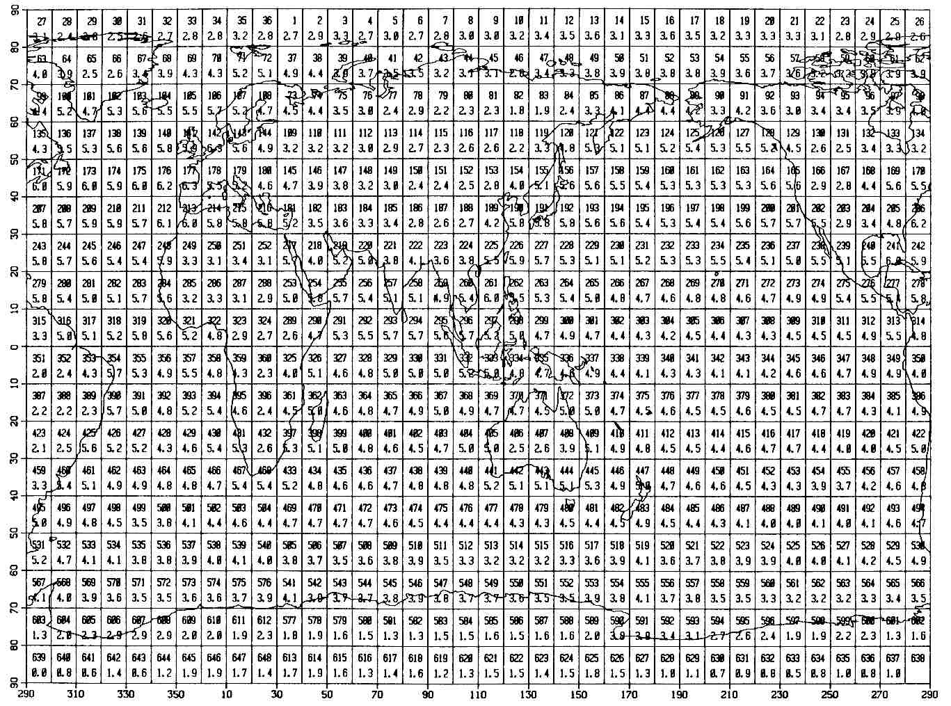
Figure 3-8. 10° boxes (smaller numerals) over log10 of reports 1854-1979 (larger numerals).
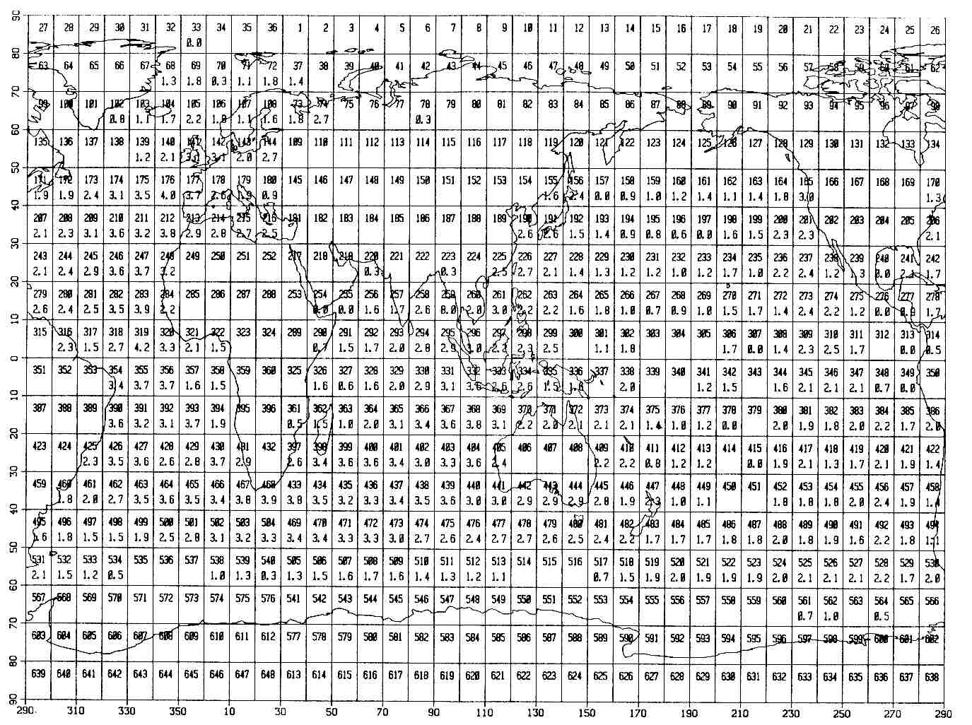
Figure 3-9. 10° boxes (smaller numerals) over log10 of reports 1854-1859 (larger numerals).

Figure 3-10. 10° boxes (smaller numerals) over log10 of reports 1860-1869 (larger numerals).
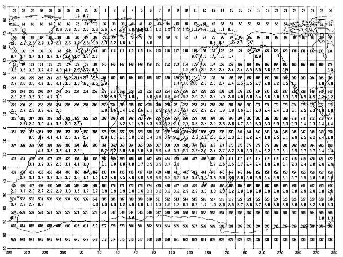
Figure 3-11. 10° boxes (smaller numerals) over log10 of reports 1870-1879 (larger numerals).
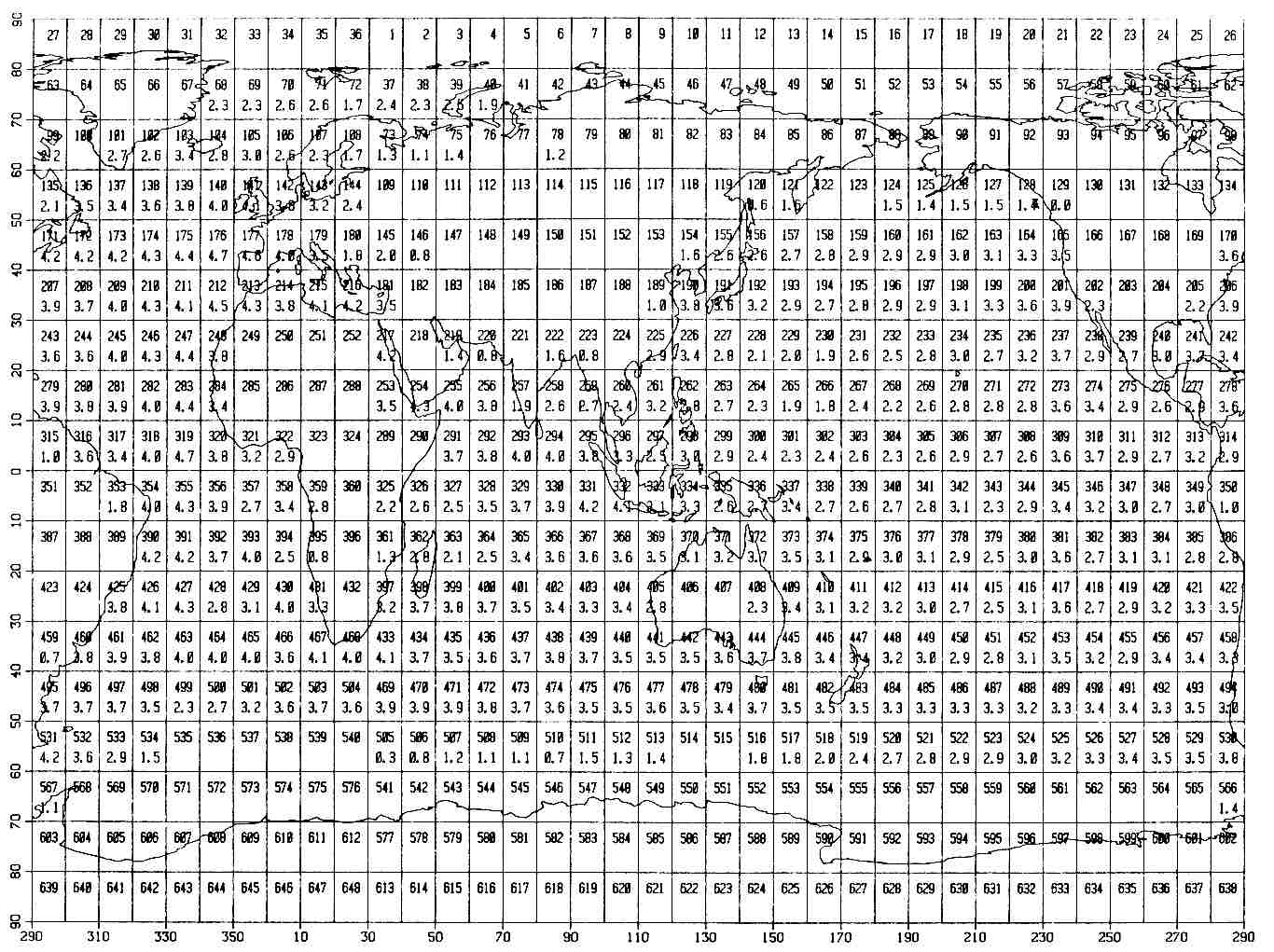
Figure 3-12. 10° boxes (smaller numerals) over log10 of reports 1880-1889 (larger numerals).
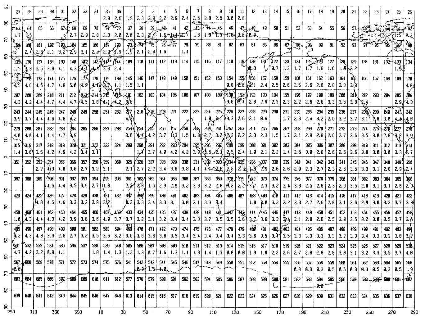
Figure 3-13. 10° boxes (smaller numerals) over log10 of reports 1890-1899 (larger numerals).

Figure 3-14. 10° boxes (smaller numerals) over log10 of reports 1900-1909 (larger numerals).
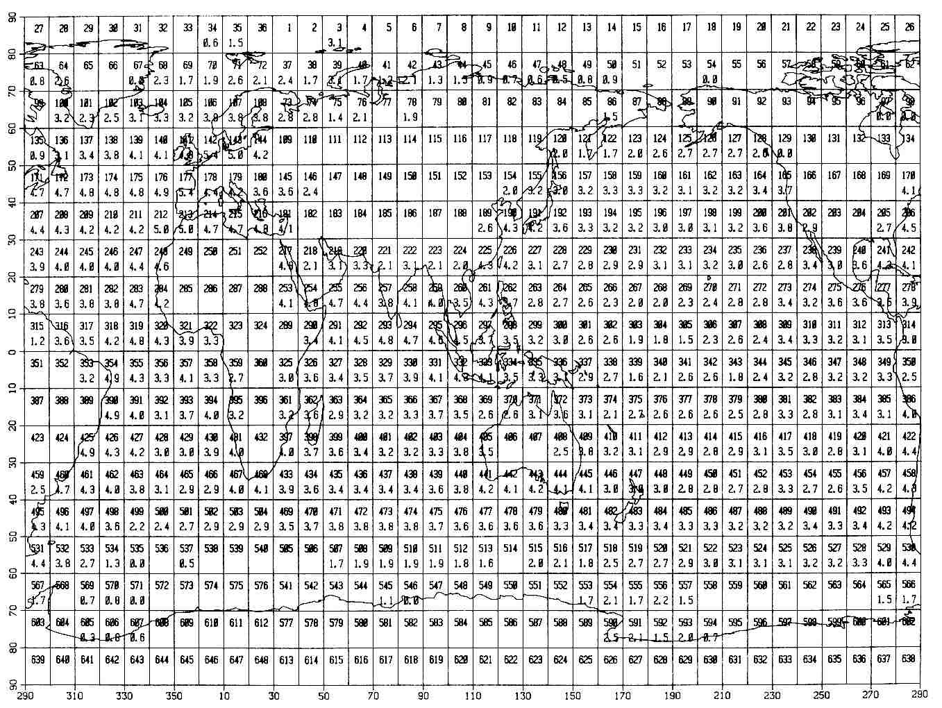
Figure 3-15. 10° boxes (smaller numerals) over log10 of reports 1910-1919 (larger numerals).
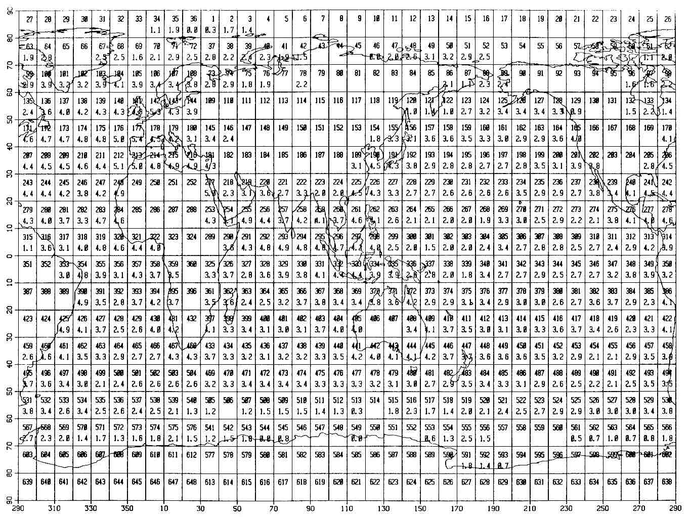
Figure 3-16. 10° boxes (smaller numerals) over log10 of reports 1920-1929 (larger numerals).
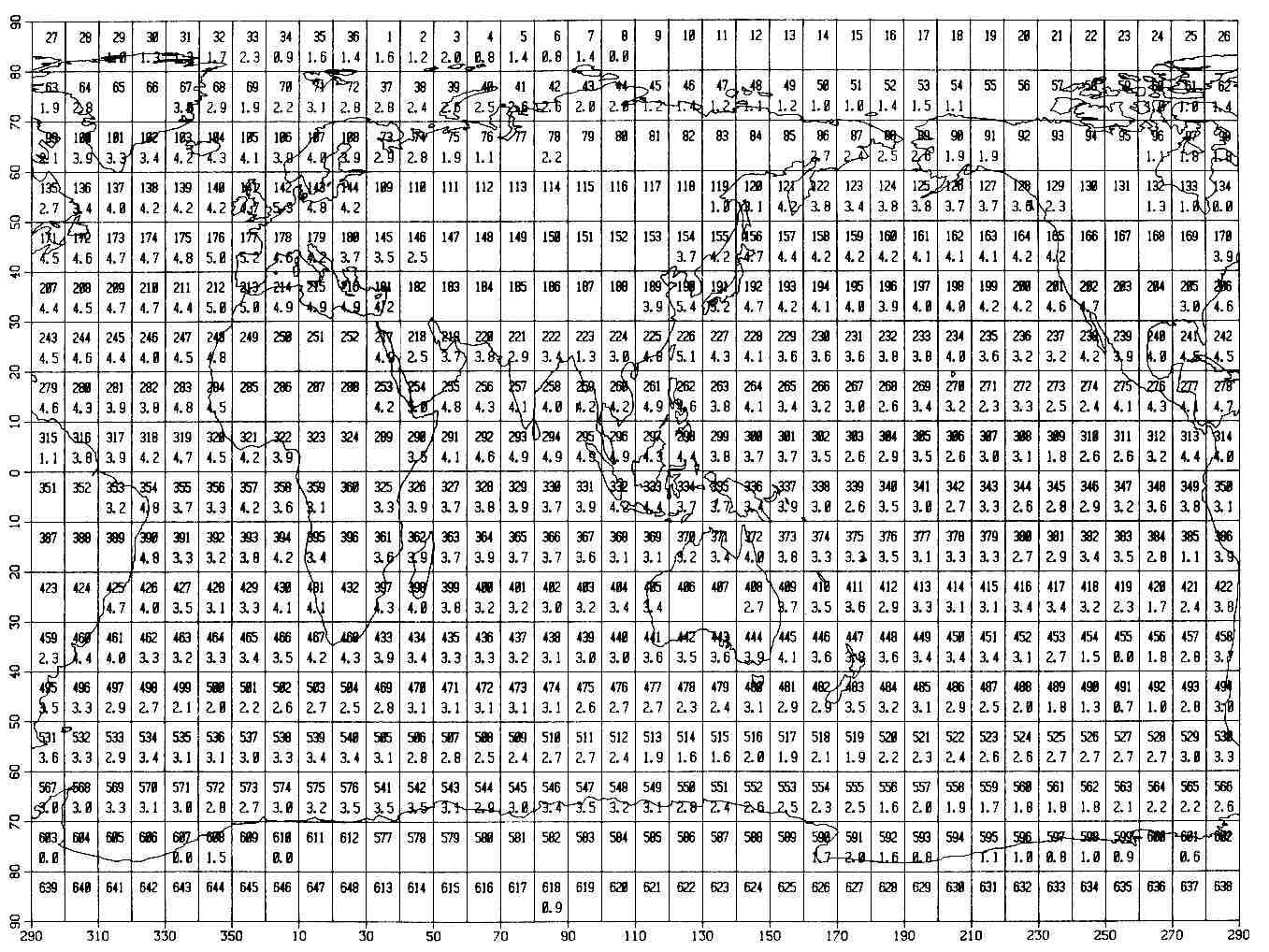
Figure 3-17. 10° boxes (smaller numerals) over log10 of reports 1930-1939 (larger numerals).
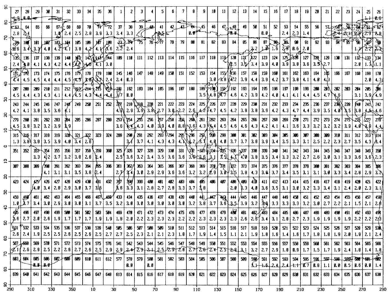
Figure 3-18. 10° boxes (smaller numerals) over log10 of reports 1940-1949 (larger numerals).
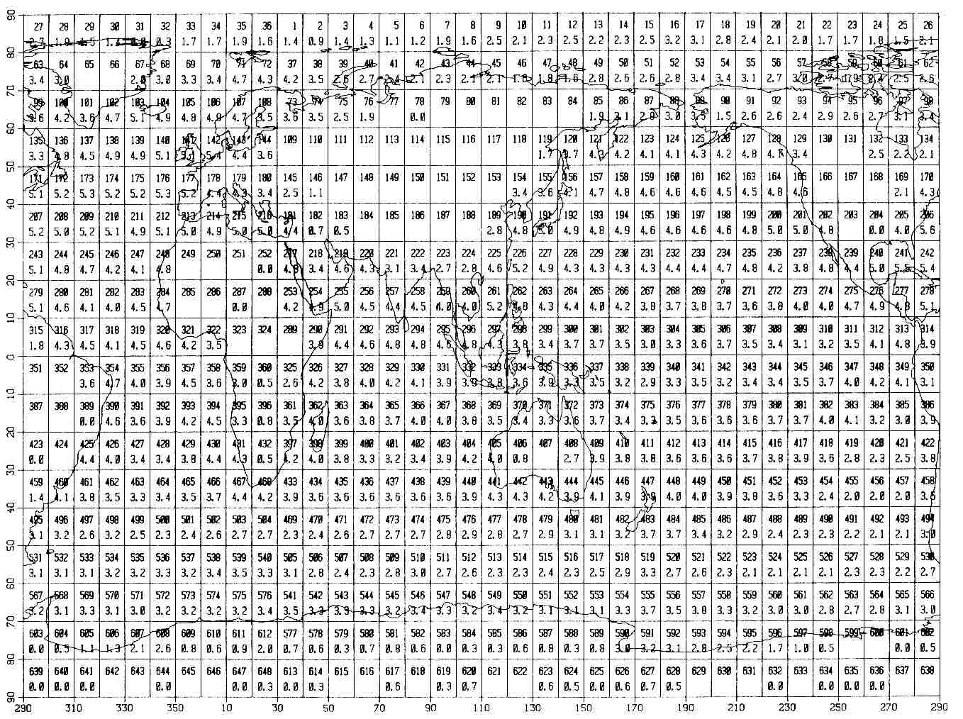
Figure 3-19. 10° boxes (smaller numerals) over log10 of reports 1950-1959 (larger numerals).
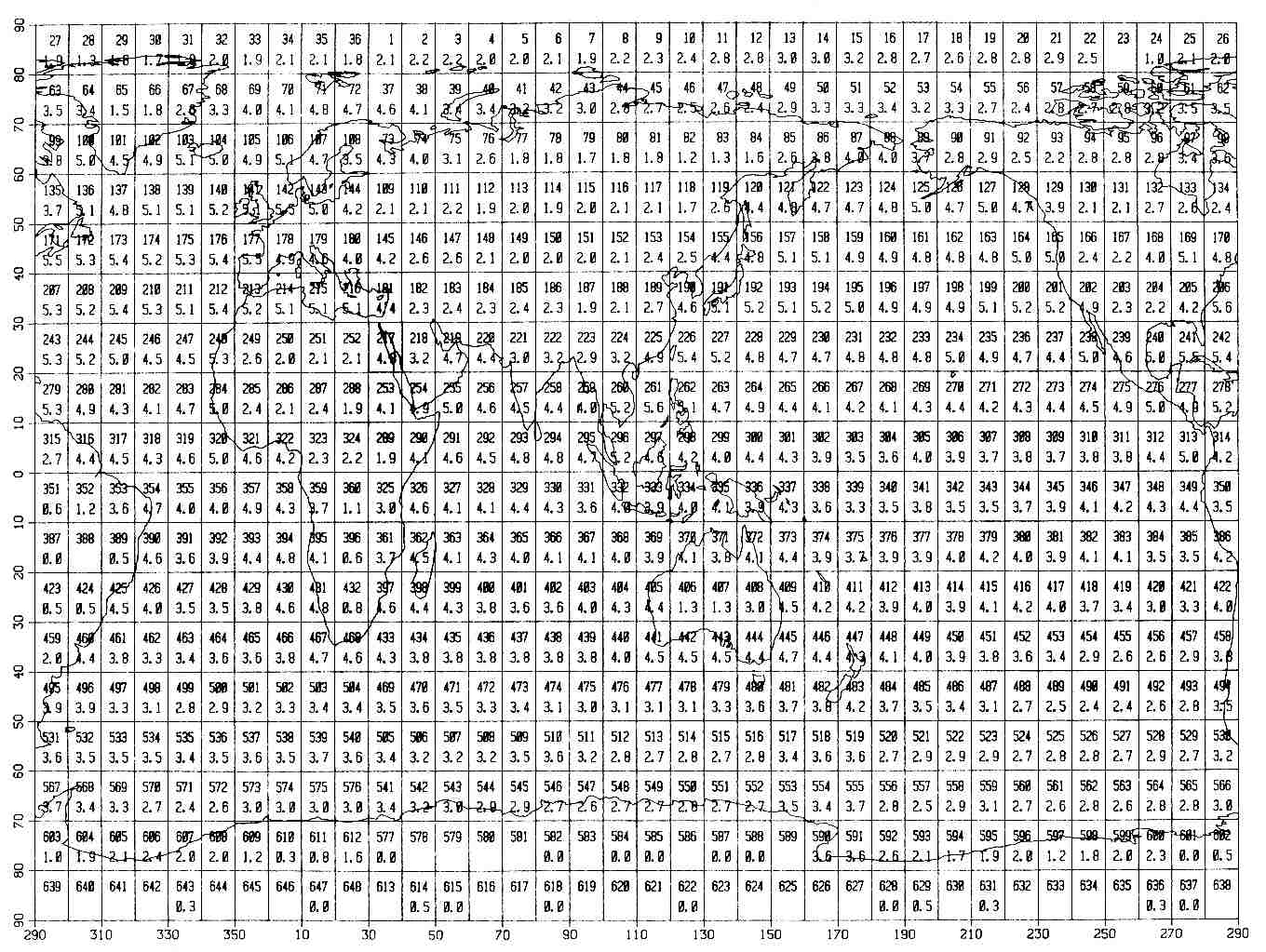
Figure 3-20. 10° boxes (smaller numerals) over log10 of reports 1960-1969 (larger numerals).

Figure 3-21. 10° boxes (smaller numerals) over log10 of reports 1970-1979 (larger numerals).
[1] Barnett, T. P., 1984: Long-term trends in surface temperature over the oceans. Mon. Wea. Rev., 112, 303-312.
[2] Environmental Science Services Administration/EDS, 1968: Climatological Data for Antarctic Stations, No. 9, January-December 1966.
[3] Jenne, R. L., and D. H. Joseph, 1974: Techniques for the processing, storage, and exchange of data. NCAR Technical Note IA-93, 46 pp. (pdf; 2.6MB)
[4] Johnson, R. A., and D. W. Wichern, 1982: Applied Multivariate Statistical Analysis, Prentice-Hall, Englewood Cliffs, NJ, 594 pp.
[5] National Climatic Data Center, 1968: TDF-11 reference manual [available from NCDC, Asheville, NC]. (pdf; 2.5MB)
[6] __________,1981 (approx.): TD-1127 reference manual [available from NCDC, Asheville, NC].
[7] __________:TD-1129(M) reference manual [available from NCDC, Asheville, NC].
[8] NOAA Data Buoy Center, 1983: Climatic summaries for NOAA data buoys [available from NDBC, NSTL Station, MS].
[9] Ramage, C. S., 1984: Can shipboard measurements reveal secular changes in tropical air-sea heat flux? J. Climate Appl. Meteor., 23, 187-193.
[10] Schlatter, T.W., and D.V. Baker, 1981: Algorithms for thermodynamic calculations. NOAA/ERL PROFS Program Office, Boulder, CO, 34 pp. [1991 version; excerpts used for COADS].
[11] U.S. Navy, 1977: Marine Climate Atlas of the World, Vol. II (Rev.), North Pacific Ocean, NAVAIR 50-1C-529, U.S. Government Printing Office, Washington, DC, 388 pp.
[12] World Meteorological Organization, 1974: Manual on Codes, Vol. 1. WMO No. 306, Geneva, Switzerland.